Step function regression in Stan
Introduction
The aim of this post is to provide a working approach to perform piecewise constant or step function regression in Stan. To set up the regression problem, consider noisy observations \(y_1, \ldots, y_n \in \mathbb{R}\) sampled from a standard signal plus i.i.d. Gaussian noise model of the form:
\[ \begin{aligned} y_i &\ = \ f(x_i) + \epsilon_i, \quad i = 1,\ldots, n \\ \epsilon_i & \overset{\text{iid}}{\sim} N(0, \sigma^2) \end{aligned} \]
with the independent variables \(x_1,\ldots, x_n \in (0, 1]\) assumed to be observed at regular (e.g. time) intervals.
The function \(f: (0,1] \to \mathbb{R}\) is unknown1, but is restricted to the space of piecewise constant functions represented as:
\[ f(x) = \sum_{k = 0}^K \mu_k \mathbb{1}\{ \gamma_{k} < x \leq \gamma_{k + 1} \} \] where \(\mathbb{1}\{x \in A\}\) denotes the indicator function and we use the convention that \(\gamma_0 = 0\) and \(\gamma_{K + 1} = 1\). Based on this representation, the regression coefficients to estimate are \(K + 1\) local means \(\mu_0,\ldots, \mu_K \in \mathbb{R}\) and \(K\) ordered breakpoints \(0 < \gamma_1 < \ldots < \gamma_{K} < 1\).
Below, we simulate a simple step function \(f(x)\) with \(K = 3\) breakpoints at regular intervals and unit valued jumps at each breakpoint. The step function \(f(x)\) is evaluated at \(x_i = i / n\) for \(i = 1,\ldots, n\) with \(n = 128\), and the noisy observations \(y_i\) are sampled from a normal distribution centered around \(f(x_i)\) with noise standard deviation \(\sigma = 0.2\).
library(ggplot2)

## parameters
K <- 3         # nr. breakpoints
N <- 128       # nr. observations
mu <- 0:K      # local means
sigma <- 0.2   # error sd

## data
set.seed(1)
f <- rep(mu, each = N / (K + 1))
x <- (1:N) / N
y <- rnorm(N, mean = f, sd = sigma)

ggplot(data = data.frame(x = x, y = y, f = f), aes(x = x)) +
  geom_line(aes(y = f), lty = 2, color = "grey50") +
  geom_point(aes(y = y)) +
  theme_light() +
  labs(x = "Time", y = "Response", title = "K = 3 breakpoints at regular intervals")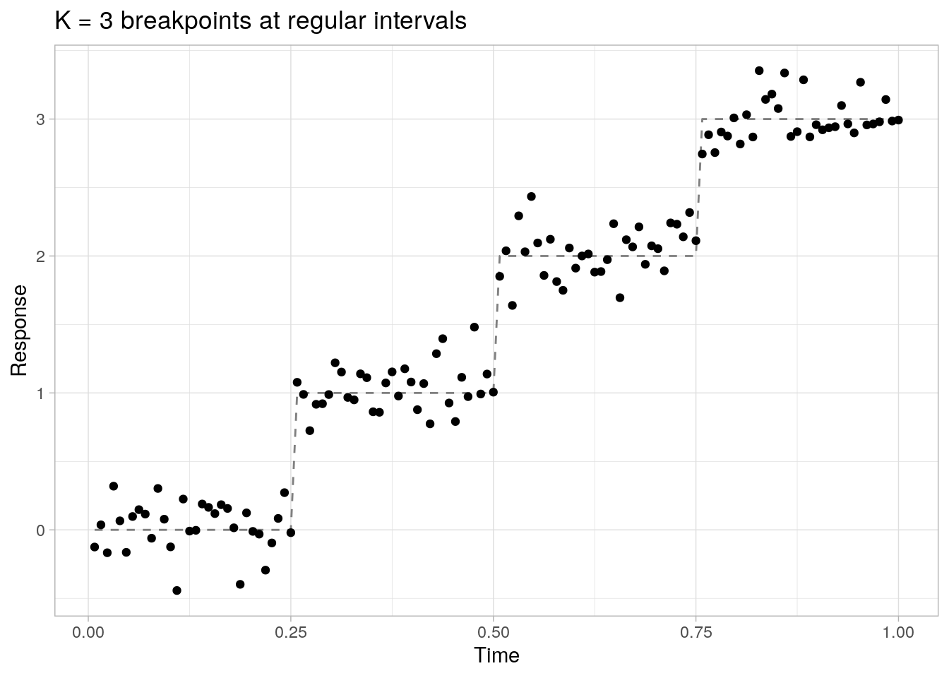
Attempt #1
In a first attempt to fit the regression model, we write a Stan program using the parameterization described above. The parameters block contains a \((K + 1)\)-dimensional vector of local means \(\boldsymbol{\mu}\), the scalar noise standard deviation \(\sigma\), and a \(K + 1\)-dimensional simplex of increments \(\tilde{\boldsymbol{\gamma}}\) (with \(K\) independent parameters), such that:
\[ \gamma_i = \sum_{k = 1}^i \tilde{\gamma}_k, \quad \text{for}\ i = 1,\ldots, K + 1 \] The breakpoint vector \(\boldsymbol{\gamma}\) itself and the regression function \(f\) are defined in the transformed parameters block. Since we have no prior knowledge on the parameter values, general weakly informative priors are specified for \(\mu\) and \(\sigma\) and a symmetric Dirichlet prior for \(\tilde{\gamma}\) corresponding to a uniform distribution on the unit simplex.
// step1.stan
data {
  int<lower=1> N;
  int<lower=1> K;
  vector[N] x;
  vector[N] y;
}
parameters {
  real mu[K + 1];
  real<lower = 0> sigma;
  simplex[K + 1] gamma_inc;
}
transformed parameters {
  vector[K + 2] gamma = append_row(0, cumulative_sum(gamma_inc));
  vector[N] f;
  for(n in 1:N) {
    for(k in 1:(K + 1)) {
      if(x[n] > gamma[k] && x[n] <= gamma[k + 1]) {
        f[n] = mu[k];
      }
    }
  }
}
model {
  mu ~ normal(0, 5);
  sigma ~ exponential(1);
  gamma_inc ~ dirichlet(rep_vector(1, K + 1));
  y ~ normal(f, sigma);
}
The Stan model compilation and HMC sampling is executed with cmdstanr, but could also be done with rstan. Below, we draw 1000 posterior samples per chain (after 1000 warm-up samples) from 4 individual chains:
library(cmdstanr)

## compile model
step1_model <- cmdstan_model("step1.stan")

## draw samples
step1_fit <- step1_model$sample(
  data = list(N = N, K = K, x = x, y =  y),
  chains = 4,
  iter_sampling = 1000,
  iter_warmup = 1000
)
#> Running MCMC with 4 sequential chains...
#>
#> Chain 1 Iteration:    1 / 2000 [  0%]  (Warmup)
#> Chain 1 Iteration:  100 / 2000 [  5%]  (Warmup)
#> Chain 1 Iteration:  200 / 2000 [ 10%]  (Warmup)
#> Chain 1 Iteration:  300 / 2000 [ 15%]  (Warmup)
#> Chain 1 Iteration:  400 / 2000 [ 20%]  (Warmup)
#> Chain 1 Iteration:  500 / 2000 [ 25%]  (Warmup)
#> Chain 1 Iteration:  600 / 2000 [ 30%]  (Warmup)
#> Chain 1 Iteration:  700 / 2000 [ 35%]  (Warmup)
#> Chain 1 Iteration:  800 / 2000 [ 40%]  (Warmup)
....
## sampling results
step1_fit
#> variable mean median sd mad q5 q95 rhat ess_bulk ess_tail
#> lp__ -105.99 -136.58 88.82 50.25 -192.73 41.93 Inf 4 NA
#> mu[1] 1.13 1.35 0.60 0.39 0.15 1.66 Inf 4 NA
#> mu[2] 0.85 0.75 0.63 0.72 0.17 1.75 Inf 4 NA
#> mu[3] 0.34 0.08 1.33 1.48 -1.05 2.23 Inf 4 NA
#> mu[4] 1.32 1.45 1.01 1.06 -0.19 2.54 Inf 4 NA
#> sigma 1.70 1.47 1.12 0.92 0.39 3.48 Inf 4 NA
#> gamma_inc[1] 0.35 0.31 0.28 0.34 0.07 0.72 Inf 4 NA
#> gamma_inc[2] 0.22 0.18 0.08 0.02 0.16 0.35 Inf 4 NA
#> gamma_inc[3] 0.24 0.17 0.21 0.15 0.04 0.58 Inf 4 NA
#> gamma_inc[4] 0.19 0.11 0.18 0.09 0.03 0.50 Inf 4 NA
#>
#> # showing 10 of 143 rows (change via 'max_rows' argument)A first look at the sampling results shows that the sampled chains completely failed to converge as indicated e.g. by the rhat column.
Calling the cmdstan_diagnose() method of the returned object, essentially all statistics indicate (extremely) poor sampling performance:
## sampling diagnostics
step1_fit$cmdstan_diagnose()
#> Processing csv files: /tmp/Rtmp4e8Bg8/step1-202106161837-1-146258.csv, /tmp/Rtmp4e8Bg8/step1-202106161837-2-146258.csv, /tmp/Rtmp4e8Bg8/step1-202106161837-3-146258.csv, /tmp/Rtmp4e8Bg8/step1-202106161837-4-146258.csv
#>
#> Checking sampler transitions treedepth.
#> 149 of 4000 (3.7%) transitions hit the maximum treedepth limit of 10, or 2^10 leapfrog steps.
#> Trajectories that are prematurely terminated due to this limit will result in slow exploration.
#> For optimal performance, increase this limit.
#>
#> Checking sampler transitions for divergences.
#> 3851 of 4000 (96%) transitions ended with a divergence.
#> These divergent transitions indicate that HMC is not fully able to explore the posterior distribution.
#> Try increasing adapt delta closer to 1.
#> If this doesn't remove all divergences, try to reparameterize the model.
#>
#> Checking E-BFMI - sampler transitions HMC potential energy.
#> The E-BFMI, 0.0039, is below the nominal threshold of 0.3 which suggests that HMC may have trouble exploring the target distribution.
#> If possible, try to reparameterize the model.
#>
#> The following parameters had fewer than 0.001 effective draws per transition:
#>   mu[1], mu[2], mu[3], mu[4], gamma_inc[2], gamma_inc[3], gamma_inc[4], gamma[3], gamma[4], f[1], f[2], f[3], f[4], f[5], f[6], f[7], f[8], f[9], f[10], f[11], f[12], f[13], f[14], f[15], f[16], f[17], f[18], f[19], f[20], f[21], f[22], f[23], f[24], f[25], f[26], f[27], f[28], f[29], f[30], f[31], f[32], f[33], f[34], f[35], f[36], f[37], f[38], f[39], f[40], f[41], f[42], f[43], f[44], f[45], f[46], f[47], f[48], f[49], f[50], f[51], f[52], f[53], f[54], f[55], f[56], f[57], f[58], f[59], f[60], f[61], f[62], f[63], f[64], f[65], f[66], f[67], f[68], f[69], f[70], f[71], f[72], f[73], f[74], f[75], f[76], f[77], f[78], f[79], f[80], f[81], f[82], f[83], f[84], f[85], f[86], f[87], f[88], f[89], f[90], f[91], f[92], f[93], f[94], f[95], f[96], f[97], f[98], f[99], f[100], f[101], f[102], f[103], f[104], f[105], f[106], f[107], f[108], f[109], f[110], f[111], f[112], f[113], f[114], f[115], f[116], f[117], f[118], f[119], f[120], f[121], f[122], f[123], f[124], f[125], f[126], f[127], f[128]
#> Such low values indicate that the effective sample size estimators may be biased high and actual performance may be substantially lower than quoted.
....
As might have already been clear already from the start, the poor sampling performance is primarily caused by the discrete jumps in \(f\) at the breakpoints \(\boldsymbol{\gamma}\), which introduce discontinuities in the gradient of the joint (log-)likelihood as specifically warned for in the Step-like functions section of Stan’s function reference.
To make this precise with an example, we explicitly write out the gradient of the joint log-likelihood when \(f\) contains a single breakpoint2, i.e. \[ f(x) = \mu_0 \mathbb{1}\{x \leq \gamma_1 \} + \mu_1 \mathbb{1}\{x > \gamma_1\} \] First, it can be verified that the likelihood of \(\boldsymbol{\theta} = (\mu_0, \mu_1, \gamma_1, \sigma)'\) conditional on \((x_i, y_i)_{i = 1}^n\) is given by:
\[ \begin{aligned} L(\boldsymbol{\theta} | \boldsymbol{x}, \boldsymbol{y}) & \ = \ \prod_{i = 1}^n \mathbb{1}\{ x_i \leq \gamma_1 \} \frac{1}{\sigma} \phi\left( \frac{y_i - \mu_0}{\sigma} \right) + \mathbb{1}\{ x_i > \gamma_1 \} \frac{1}{\sigma} \phi\left( \frac{y_i - \mu_1}{\sigma} \right) \\ & \ = \ \prod_{i=1}^n \frac{1}{\sigma} \phi\left( \frac{y_i - (\mu_0 + (\mu_1 - \mu_0) \mathbb{1}\{ x_i > \gamma_1 \})}{\sigma} \right) \end{aligned} \] where \(\phi\) denotes the probability density function of a standard normal. Taking the logarithm of the right-hand side produces the joint log-likelihood:
\[ \begin{aligned} \ell(\boldsymbol{\theta} | \boldsymbol{x}, \boldsymbol{y}) & \ = \ -\frac{n}{2} \log(2\pi\sigma^2) - \frac{1}{2\sigma^2}\sum_{i = 1}^n (y_i - (\mu_0 + (\mu_1 - \mu_0)\mathbb{1}\{x_i > \gamma_1\}))^2 \end{aligned} \]
and the derivatives of the log-likelihood with respect to \(\mu_0, \mu_1, \sigma\) are given by:
\[ \begin{aligned} \frac{\partial \ell}{\partial \mu_0} & \ = \ \frac{1}{\sigma^2} \sum_{i = 1}^n (y_i - \mu_0)\mathbb{1}\{ x_i \leq \gamma_1 \}\\ \frac{\partial \ell}{\partial \mu_1} & \ = \ \frac{1}{\sigma^2} \sum_{i = 1}^n (y_i - \mu_1)\mathbb{1}\{ x_i > \gamma_1 \}\\ \frac{\partial \ell}{\partial \sigma} & \ = \ \frac{n}{\sigma} + \frac{1}{\sigma^3}\sum_{i = 1}^n (y_i - (\mu_0 + (\mu_1 - \mu_0)\mathbb{1}\{x_i > \gamma_1\}))^2 \end{aligned} \] The derivative of the log-likelihood with respect to \(\gamma_1\) does not exist at \(\{ x_1,\ldots,x_n \}\) (as \(\ell(\gamma_1)\) is discontinuous at these points) and is zero everywhere else.
Suppose that \(\gamma_1\) would be known and no longer needs to be estimated. Then the gradient of the log-likelihood consists only of the three partial derivatives listed above, which exist everywhere and are in fact continuous in each marginal direction. Note that this assumption does not make \(f\) continuous as a function of \(x\), but that does not matter, only the continuity of the gradient matters in order to improves Stan’s sampling performance.
Below, we recompile the Stan model by removing the parameter vector \(\tilde{\boldsymbol{\gamma}}\) and replacing the breakpoints \(\boldsymbol{\gamma}\) by their true (unknown) values:
// step1a.stan
data {
  int<lower=1> N;
  int<lower=1> K;
  vector[N] x;
  vector[N] y;
}
transformed data{
  simplex[K + 1] gamma_inc = rep_vector(0.25, 4);
}
parameters {
  real mu[K + 1];
  real<lower = 0> sigma;
}
transformed parameters {
  vector[K + 2] gamma = append_row(0, cumulative_sum(gamma_inc));
  vector[N] f;
  for(n in 1:N) {
    for(k in 1:(K + 1)) {
      if(x[n] > gamma[k] && x[n] <= gamma[k + 1]) {
        f[n] = mu[k];
      }
    }
  }
}
model {
  mu ~ normal(0, 5);
  sigma ~ exponential(1);
  y ~ normal(f, sigma);
}
We redraw 4000 posterior samples across 4 chains with cmdstanr as before:
## recompile model
step1a_model <- cmdstan_model("step1a.stan")

## redraw samples
step1a_fit <- step1a_model$sample(
  data = list(N = N, K = K, x = x, y =  y),
  chains = 4,
  iter_sampling = 1000,
  iter_warmup = 1000
)
#> Running MCMC with 4 sequential chains...
#>
#> Chain 1 Iteration:    1 / 2000 [  0%]  (Warmup)
#> Chain 1 Iteration:  100 / 2000 [  5%]  (Warmup)
#> Chain 1 Iteration:  200 / 2000 [ 10%]  (Warmup)
#> Chain 1 Iteration:  300 / 2000 [ 15%]  (Warmup)
#> Chain 1 Iteration:  400 / 2000 [ 20%]  (Warmup)
#> Chain 1 Iteration:  500 / 2000 [ 25%]  (Warmup)
#> Chain 1 Iteration:  600 / 2000 [ 30%]  (Warmup)
#> Chain 1 Iteration:  700 / 2000 [ 35%]  (Warmup)
#> Chain 1 Iteration:  800 / 2000 [ 40%]  (Warmup)
....
As expected, the sampling results are much more satisfactory than before:
## sampling results
step1a_fit
#>  variable   mean median   sd  mad     q5    q95 rhat ess_bulk ess_tail
#>  lp__     156.69 157.04 1.69 1.49 153.34 158.72 1.00     2006     2418
#>  mu[1]      0.02   0.02 0.03 0.03  -0.03   0.08 1.00     5077     2661
#>  mu[2]      1.04   1.04 0.03 0.03   0.98   1.09 1.00     5144     2942
#>  mu[3]      2.03   2.03 0.03 0.03   1.98   2.08 1.00     5629     3007
#>  mu[4]      3.00   3.00 0.03 0.03   2.95   3.05 1.00     5126     2740
#>  sigma      0.18   0.18 0.01 0.01   0.16   0.20 1.00     4458     2698
#>  gamma[1]   0.00   0.00 0.00 0.00   0.00   0.00   NA       NA       NA
#>  gamma[2]   0.25   0.25 0.00 0.00   0.25   0.25   NA       NA       NA
#>  gamma[3]   0.50   0.50 0.00 0.00   0.50   0.50   NA       NA       NA
#>  gamma[4]   0.75   0.75 0.00 0.00   0.75   0.75   NA       NA       NA
#>
#>  # showing 10 of 139 rows (change via 'max_rows' argument)
## sampling diagnostics
step1a_fit$cmdstan_diagnose()
#> Processing csv files: /tmp/Rtmp4e8Bg8/step1a-202106161837-1-36be58.csv, /tmp/Rtmp4e8Bg8/step1a-202106161837-2-36be58.csv, /tmp/Rtmp4e8Bg8/step1a-202106161837-3-36be58.csv, /tmp/Rtmp4e8Bg8/step1a-202106161837-4-36be58.csv
#>
#> Checking sampler transitions treedepth.
#> Treedepth satisfactory for all transitions.
#>
#> Checking sampler transitions for divergences.
#> No divergent transitions found.
#>
#> Checking E-BFMI - sampler transitions HMC potential energy.
#> E-BFMI satisfactory for all transitions.
#>
#> Effective sample size satisfactory.
#>
#> Split R-hat values satisfactory all parameters.
#>
#> Processing complete, no problems detected.Obviously, the breakpoints \(\boldsymbol{\gamma}\) cannot assumed to be known in advance, but the previous example does highlight the fact that the Stan model should be reparameterized in such a way that the discontinuous indicator functions do not depend on the unknown parameters to make sure that the gradient of the joint log-likelihood exists and is continuous.
Attempt #2
In a second attempt, we no longer try to explicitly model the breakpoint parameters \(\boldsymbol{\gamma}\). Instead, the idea is to allow for a possible discrete jump at every location \(x_i\) for \(i = 1, \ldots, n\). Without any type of regularization, such a model would be heavily overparameterized requiring the same number of parameters as the number of observations. However, the function \(f(x)\) is piecewise constant, so we can use the fact that most jump sizes are actually zero and only few non-zero jumps should be sufficient to capture the behavior of \(f(x)\).
Discrete Haar wavelet transform
To make this idea concrete, we will decompose the input vector \(y_1,\ldots,y_n\) according to a discrete Haar wavelet transform, which is a linear transformation that expands the \(n\)-dimensional input vector \(y_1,\ldots,y_n\) into an \((n-1)\)-dimensional vector of wavelet (or difference) coefficients \(d_1,\ldots,d_{n-1}\) and a single scaling (or average) coefficient \(c_0\). The discrete Haar wavelet transform is the most basic wavelet transform and is particularly well-suited to decompose piecewise constant signals, which generally produce very sparse Haar wavelet coefficient vectors with most wavelet coefficients equal to zero. For a description of the discrete Haar wavelet transform and a more general introduction to the use of wavelets in statistics, see e.g. (Nason 2008) or (Jansen 2012).
For simplicity, in the remainder of this post it is assumed that the number of observations is dyadic, i.e. \(n = 2^J\) for some integer \(J\), which is a common assumption in the context of wavelet regression3. Given the input signal \(f(x_1),\ldots,f(x_n)\), it is quite straightforward to encode the forward Haar transform in a recursive fashion:
## helper function to calculate scaling (average) or wavelet (difference) coefficients
filt <- function(C, fun) fun(C[c(T, F)], C[c(F, T)]) / sqrt(2)

## lists with scaling + wavelet coefficients from course to fine scales
C <- D <- vector(mode = "list", length = log2(N))

## recursively update course scale coefficients
for(l in log2(N):1) {
  C[[l]] <- filt(C = if(l < log2(N)) C[[l + 1]] else f, fun = `+`)
  D[[l]] <- filt(C = if(l < log2(N)) C[[l + 1]] else f, fun = `-`)
}
The list with scaling coefficients C consists of scaled local averages at increasingly coarse resolution scales, with the scaling coefficient at the coarsest scale (i.e. C[[1]]) being equivalent to the global mean scaled by a known factor:
all.equal(C[[1]], 2^(log2(N)/2) * mean(f))
#> [1] TRUE
Analogously, the list with wavelet coefficients D consists of scaled local differences of the scaling coefficients at increasingly coarse resolution scales. For the piecewise constant signal f, the list of wavelet coefficients is very sparse as most local differences are equal to zero and only a few non-zero wavelet coefficients are necessary to encode the jumps in the signal4:
D
#> [[1]]
#> [1] -11.31371
#>
#> [[2]]
#> [1] -4 -4
#>
#> [[3]]
#> [1] 0 0 0 0
#>
#> [[4]]
#> [1] 0 0 0 0 0 0 0 0
#>
#> [[5]]
#>  [1] 0 0 0 0 0 0 0 0 0 0 0 0 0 0 0 0
#>
#> [[6]]
#>  [1] 0 0 0 0 0 0 0 0 0 0 0 0 0 0 0 0 0 0 0 0 0 0 0 0 0 0 0 0 0 0 0 0
#>
#> [[7]]
#>  [1] 0 0 0 0 0 0 0 0 0 0 0 0 0 0 0 0 0 0 0 0 0 0 0 0 0 0 0 0 0 0 0 0 0 0 0 0 0 0
#> [39] 0 0 0 0 0 0 0 0 0 0 0 0 0 0 0 0 0 0 0 0 0 0 0 0 0 0
Keeping track of all scaling and wavelet coefficients contained in C and D is redundant. To reconstruct the original input signal we need only the coarsest scaling coefficient C[[1]] and the \(n-1\) wavelet coefficients present in D. The inverse (or backward) Haar wavelet transform follows directly by applying the average and difference operations in the forward wavelet transform in the opposite sense:
## helper function to reconstruct scaling coefficients at finer scale
inv_filt <- function(C, D) c(t(cbind((C + D) / sqrt(2), (C - D) / sqrt(2))))

## recursively reconstruct fine scale coefficients
f1 <- C[[1]]
for(l in 1:log2(N)) {
  f1 <- inv_filt(C = f1, D = D[[l]])
}

all.equal(f, f1)
#> [1] TRUE
The following functions encode the discrete (forward and backward) Haar wavelet transform in Stan and are saved in a file named haar.stan:
// haar.stan

// filter C coefficient vector
vector filtC(vector C, int N) {
    vector[N] C1;
    for (n in 1 : N) {
        C1[n] = (C[2 * n - 1] + C[2 * n]) / sqrt2();
    }
    return C1;
}
// filter D coefficient vector
vector filtD(vector D, int N) {
    vector[N] D1;
    for (n in 1 : N) {
        D1[n] = (D[2 * n - 1] - D[2 * n]) / sqrt2();
    }
    return D1;
}
// reconstruct C coefficient vector
vector inv_filt(vector C, vector D, int N) {
    vector[2 * N] C1;
    for (n in 1 : N) {
        C1[2 * n - 1] = (C[n] + D[n]) / sqrt2();
        C1[2 * n] = (C[n] - D[n]) / sqrt2();
    }
    return C1;
}
// forward Haar wavelet transform
vector fwt(vector y) {
    int N = rows(y);
    int Ni = 0;
    vector[N] ywd;
    vector[N] C = y;
    while (N > 1) {
        N /= 2;
        ywd[(Ni + 1):(Ni + N)] = filtD(C[1 : (2 * N)], N);
        C[1:N] = filtC(C[1 : (2 * N)], N);
        Ni += N;
    }
    ywd[Ni + 1] = C[1];
    return ywd;
}
// inverse Haar wavelet transform
vector iwt(vector ywd) {
    int N = rows(ywd);
    vector[N] y;
    int Nj = 1;
    y[1] = ywd[N];
    while (Nj < N) {
        y [1 : (2 * Nj)] = inv_filt(y[1 : Nj], ywd[(N - 2 * Nj + 1) : (N - Nj)], Nj);
        Nj *= 2;
    }
    return y;
}
The above code can then easily be included in the functions block of another Stan file with #include haar.stan. For instance, we can verify that the forward and backward wavelet transforms produce the expected outputs:
// haar_test.stan
functions{
  #include haar.stan
}
data {
  int<lower=1> N;
  vector[N] y;
}
parameters {
}
generated quantities {
   vector[N] ywd = fwt(y);
   vector[N] y1 = iwt(ywd);
}
## compile model
dwt_model <- cmdstan_model("haar_test.stan", include_paths = ".")
## draw single sample with no parameters
dwt_fit <- dwt_model$sample(
data = list(N = N, y = f),
chains = 1,
iter_sampling = 1,
iter_warmup = 0,
sig_figs = 18,
fixed_param = TRUE
)
#> Running MCMC with 1 chain...
#>
#> Chain 1 Iteration: 1 / 1 [100%] (Sampling)
#> Chain 1 finished in 0.0 seconds.
## check forward wavelet transform
all.equal(c(dwt_fit$draws(variables = "ywd")), c(unlist(rev(D)), C[[1]]))
#> [1] TRUE
## check inverse wavelet transform
all.equal(c(dwt_fit$draws(variables = "y1")), f)
#> [1] TRUEWavelet domain regression
Provided that the target signal \(f(x)\) has a sparse representation in the wavelet domain, a sensible estimation approach is to: (1) transform the noisy observation vector \(\boldsymbol{y} = (y_1,\ldots,y_n)'\) to the wavelet domain; (2) perform a sparse regression on the wavelet coefficients; (3) transform the result back to the functional domain to obtain an estimate \(\hat{f}(x)\).
As mentioned previously, the discrete Haar wavelet transform is a linear transformation \(\boldsymbol{d}^y = \boldsymbol{W} \boldsymbol{y}\), with \((n \times n)\)-dimensional wavelet transformation matrix \(\boldsymbol{W}\). Given the signal plus i.i.d. Gaussian noise model for the observations, \[ \boldsymbol{y} \ \sim N(\boldsymbol{f}, \sigma^2\boldsymbol{I}_{n \times n}) \] this implies that the transformed observations in the wavelet domain also follow a Gaussian signal plus noise model: \[ \boldsymbol{d}^y \ \sim N(\boldsymbol{d}^f, \sigma^2 \boldsymbol{W}\boldsymbol{W}') \] where \(\boldsymbol{d}^f = \boldsymbol{W}\boldsymbol{f}\) is the wavelet transformation of the target signal \(\boldsymbol{f} = (f(x_1),\ldots,f(x_n))'\).
Moreover, the linear transformation matrix \(\boldsymbol{W}\) is a unitary matrix, i.e. the transpose \(\boldsymbol{W}'\) and the inverse \(\boldsymbol{W}^{-1}\) coincide, (see e.g. (Nason 2008, Ch. 2)). This is particularly useful as it means that we also have a signal plus i.i.d. Gaussian noise model in the wavelet domain with the same noise variance as in the functional domain:
\[ d^y_{i} \ \overset{\text{iid}}{\sim} N(d^f_{i}, \sigma^2), \quad i = 1,\ldots, n \]
That is, the regression problem in the wavelet domain comes down to sparse linear regression in an i.i.d. Gaussian noise model.
Sparse linear regression in Stan
To induce sparsity in the estimated wavelet coefficient vector, we use a simplified version of the Finnish horseshoe prior as described in (Betancourt 2018), which is summarized as:
\[ \begin{aligned} d^f_i & \sim \ N(0, \tilde{\lambda}_i^2 ) \\ \tilde{\lambda}_i & \ = \ \frac{\tau \lambda_i}{\sqrt{1 + \tau^2 \lambda_i^2}} \\ \lambda_i & \sim \ \text{Half-}\mathcal{C}(0, 1) \\ \tau & \sim \ \text{Half-}N(0, \tau_0) \end{aligned} \]
The difference with respect to the specification in (Betancourt 2018) is that the additional scale parameter \(c\) is set to 1 and the Cauchy prior for \(\tau\) is replaced by a light-tailed normal prior. The \(\tau_0\) parameter is calculated as:
\[ \tau_0 \ = \ \frac{m_0}{1 - m_0} \frac{\sigma_0}{\sqrt{N}} \] where \(m_0\) is the expected fraction of non-zero wavelet coefficients (provided as input data), and \(\sigma_0\) is an initial estimate of the noise variance. The value for \(\sigma_0\) is calculated automatically by taking the standard deviation of the finest-scale coefficients in the noisy vector \(\boldsymbol{d}^y\), which are expected to contain primarily noise and (almost) no signal. As in (Betancourt 2018), the sampling results are not very sensitive to the value of \(m_0\) (and consequently \(\tau_0\)), but it does provide a convenient global tuning parameter for the amount of regularization applied to the estimated coefficients.
The complete model is encoded in a new Stan file step2.stan. First, the input vector \(y\) is transformed to the wavelet domain (ywd) in the transformed data block. The wavelet coefficient vector of the target signal \(f\) is constructed in the transformed parameters block based on the considerations above. To reduce the number of model parameters, the wavelet coefficients at the finest resolution scale are directly set to zero, (as the finest-scale wavelet coefficients are expected to contain only noise), leaving a set of \(N/2 - 1\) (sparse) wavelet coefficients to be estimated. The model block specifies the simplified Finnish horseshoe priors as well as a naive normal prior for the noise standard deviation \(\sigma\). In addition, the likelihood contributions based on the wavelet domain Gaussian linear model are specified. Finally, the regularized wavelet coefficient vector is back-transformed to the functional domain in the generated quantities block.
// step2.stan
functions{
  #include haar.stan
}
data {
  int<lower=1> N;
  vector[N] y;        // input vector
  real<lower = 0> m0; // expected fraction of non-zero coefficients
}
transformed data{
  int M = (N / 2) - 1;                               // # estimated coefficients
  vector[N] ywd = fwt(y);                            // wavelet coefficients input
  real sigma0 = sd(ywd[1 : (N / 2)]);                // initial estimate sigma
  real tau0 = m0 / (1 - m0) * sigma0 / sqrt(N - 1);  // irrelevance scale
}
parameters {
  real<lower=0> sigma;        // noise standard deviation
  real<lower=0> tau;          // global scale horseshoe
  vector[M] z;                // unscaled estimated coefficients
  vector<lower=0>[M] lambda;  // local scales horseshoe
}
transformed parameters {
  // regularized (sparse) wavelet coefficients
  vector[N] fwd = rep_vector(0.0, N);
  fwd[(N - M) : (N - 1)] = (tau * lambda ./ sqrt(1 + square(tau * lambda))) .* z;
  fwd[N] = ywd[N];
}
model {
  // (sparse) priors
  lambda ~ cauchy(0, 1);
  sigma ~ normal(sigma0, 5 * sigma0);
  tau ~ normal(0, tau0);
  z ~ std_normal();
  // likelhood contributions
  ywd[1 : (N - 1)] ~ normal(fwd[1 : (N - 1)], sigma);
}
generated quantities {
  // back-transformed coefficients
  vector[N] f = iwt(fwd);
}
We compile the model with cmdstanr and draw 1000 (after 1000 warm-up samples) per chain from 4 individual chains as before. For the expected fraction of non-zero wavelet coefficients, we use \(m_0 = 0.05\), which is quite conservative given our prior knowledge on the sparseness of the signal.
## compile model
step2_model <- cmdstan_model("step2.stan", include_paths = ".")

## draw samples
step2_fit <- step2_model$sample(
  data = list(N = N, y = y, m0 = 0.05),
  chains = 4,
  iter_sampling = 1000,
  iter_warmup = 1000
)
#> Running MCMC with 4 sequential chains...
#>
#> Chain 1 Iteration:    1 / 2000 [  0%]  (Warmup)
#> Chain 1 Iteration:  100 / 2000 [  5%]  (Warmup)
#> Chain 1 Iteration:  200 / 2000 [ 10%]  (Warmup)
#> Chain 1 Iteration:  300 / 2000 [ 15%]  (Warmup)
#> Chain 1 Iteration:  400 / 2000 [ 20%]  (Warmup)
#> Chain 1 Iteration:  500 / 2000 [ 25%]  (Warmup)
#> Chain 1 Iteration:  600 / 2000 [ 30%]  (Warmup)
#> Chain 1 Iteration:  700 / 2000 [ 35%]  (Warmup)
#> Chain 1 Iteration:  800 / 2000 [ 40%]  (Warmup)
....
## sampling results
step2_fit
#> variable mean median sd mad q5 q95 rhat ess_bulk ess_tail
#> lp__ -69.75 -69.58 9.20 9.44 -85.25 -55.05 1.00 1084 1954
#> sigma 0.18 0.18 0.01 0.01 0.16 0.20 1.00 4411 3292
#> tau 0.00 0.00 0.00 0.00 0.00 0.00 1.00 4376 2659
#> z[1] -0.04 -0.05 1.01 1.01 -1.63 1.61 1.00 6083 2605
#> z[2] -0.04 -0.05 1.00 0.97 -1.65 1.59 1.00 6483 2697
#> z[3] 0.00 -0.02 1.04 1.05 -1.69 1.70 1.00 5897 2130
#> z[4] -0.06 -0.08 1.04 1.07 -1.74 1.65 1.00 5885 2644
#> z[5] -0.02 -0.02 1.01 1.00 -1.70 1.61 1.00 6283 2566
#> z[6] 0.07 0.06 0.99 1.00 -1.53 1.68 1.00 5923 2462
#> z[7] 0.02 0.01 1.01 1.01 -1.62 1.67 1.00 6808 2943
#>
#> # showing 10 of 385 rows (change via 'max_rows' argument)## sampling diagnostics
step2_fit$cmdstan_diagnose()
#> Processing csv files: /tmp/Rtmp4e8Bg8/step2-202106161838-1-186086.csv, /tmp/Rtmp4e8Bg8/step2-202106161838-2-186086.csv, /tmp/Rtmp4e8Bg8/step2-202106161838-3-186086.csv, /tmp/Rtmp4e8Bg8/step2-202106161838-4-186086.csv
#>
#> Checking sampler transitions treedepth.
#> Treedepth satisfactory for all transitions.
#>
#> Checking sampler transitions for divergences.
#> No divergent transitions found.
#>
#> Checking E-BFMI - sampler transitions HMC potential energy.
#> E-BFMI satisfactory for all transitions.
#>
#> Effective sample size satisfactory.
#>
#> Split R-hat values satisfactory all parameters.
#>
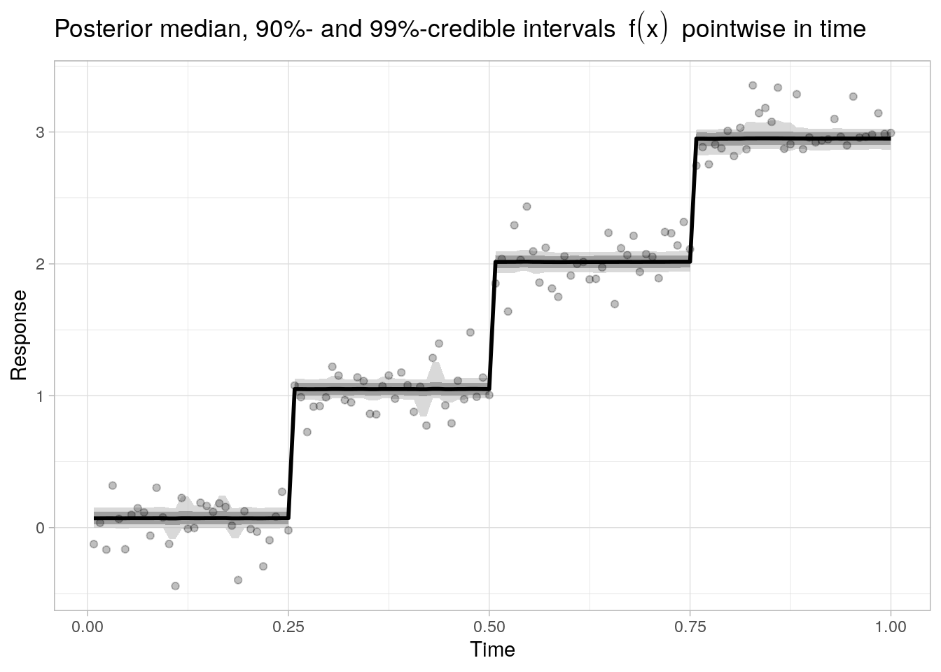
#> Processing complete, no problems detected.In contrast to the first estimation attempt in step1.stan, the sampling diagnostics now produce satisfying results as we have reparametrized the model to avoid the problematic log-likelihood gradient.
Below, we plot the posterior median of \(f\) as well as 90%- and 99%-credible bands (pointwise in time):
Blocks test function
To conclude, we apply the same sampling procedure to a more challenging example using the blocks test function available through DJ.EX() in the wavethresh-package, see also (Nason 2008, Ch. 3). The observations \(y_1, \ldots, y_n\) with \(n = 256\) are sampled from a signal plus i.i.d. Gaussian noise model as before:
library(wavethresh)
## data
set.seed(1)
N <- 256
x <- (1:N) / N
f <- DJ.EX(n = N, signal = 1)$blocks
y <- DJ.EX(n = N, signal = 1, rsnr = 5, noisy = TRUE)$blocks
ggplot(data = data.frame(x = x, y = y, f = f), aes(x = x)) +
geom_line(aes(y = f), lty = 2, color = "grey50") +
geom_point(aes(y = y)) +
theme_light() +
labs(x = "Time", y = "Response", title = "Blocks test function with i.i.d. Gaussian noise (N = 256)")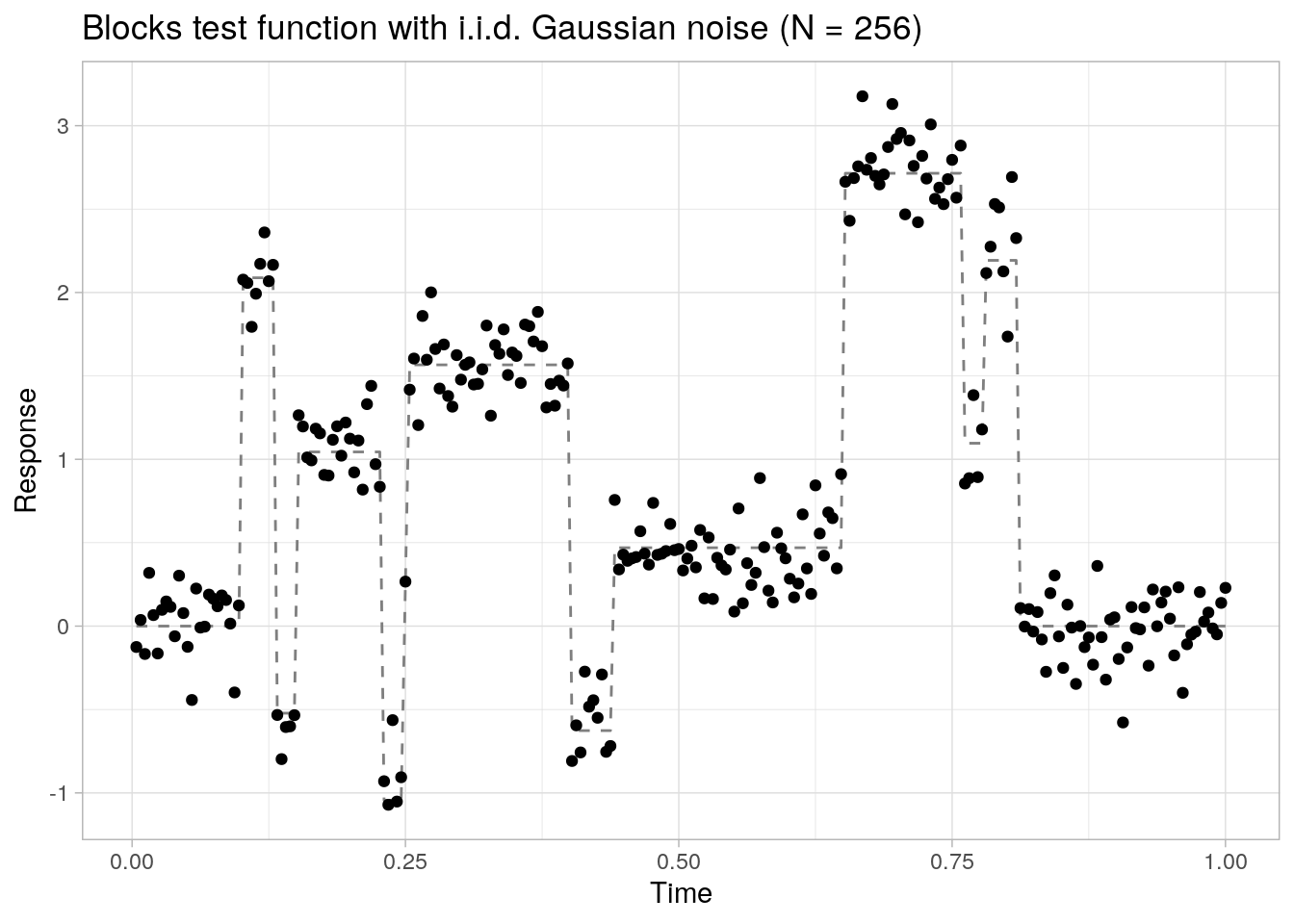 We draw 1000 posterior samples (after 1000 warm-up samples) per chain from 4 individual chains, with the expected fraction of non-zero wavelet coefficients set to \(m_0 = 0.05\) as before. Note that the number of breakpoints present in the signal does not need to be known prior to fitting the model.
## draw samples
blocks_fit <- step2_model$sample(
data = list(N = N, y = y, m0 = 0.05),
chains = 4,
iter_sampling = 1000,
iter_warmup = 1000
)
#> Running MCMC with 4 sequential chains...
#>
#> Chain 1 Iteration: 1 / 2000 [ 0%] (Warmup)
#> Chain 1 Iteration: 100 / 2000 [ 5%] (Warmup)
#> Chain 1 Iteration: 200 / 2000 [ 10%] (Warmup)
#> Chain 1 Iteration: 300 / 2000 [ 15%] (Warmup)
#> Chain 1 Iteration: 400 / 2000 [ 20%] (Warmup)
#> Chain 1 Iteration: 500 / 2000 [ 25%] (Warmup)
#> Chain 1 Iteration: 600 / 2000 [ 30%] (Warmup)
#> Chain 1 Iteration: 700 / 2000 [ 35%] (Warmup)
#> Chain 1 Iteration: 800 / 2000 [ 40%] (Warmup)
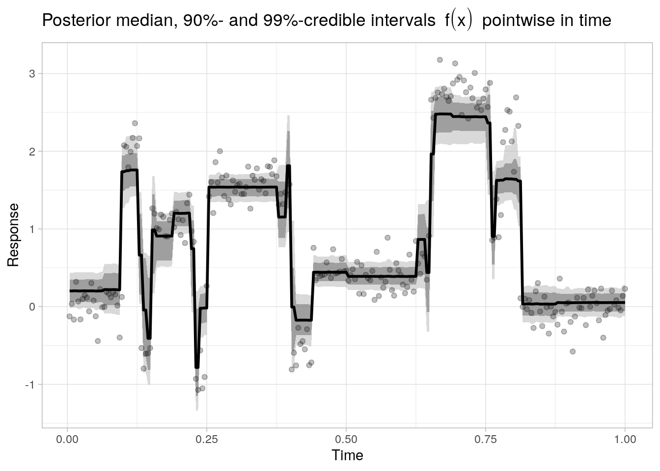
....The sampling results and diagnostics all look satisfactory:
## sampling results
blocks_fit
#>  variable    mean  median    sd   mad      q5     q95 rhat ess_bulk ess_tail
#>     lp__  -330.02 -329.62 13.39 13.15 -352.96 -308.54 1.00      436     1860
#>     sigma    0.38    0.38  0.04  0.03    0.33    0.45 1.01      126      239
#>     tau      0.00    0.00  0.00  0.00    0.00    0.01 1.00     1181     1866
#>     z[1]    -0.02    0.00  1.02  1.00   -1.71    1.66 1.00     6564     2765
#>     z[2]    -0.02   -0.03  1.00  1.01   -1.65    1.63 1.00     6298     2965
#>     z[3]    -0.01   -0.02  0.96  0.96   -1.58    1.57 1.00     5677     2899
#>     z[4]    -0.04   -0.06  1.02  1.03   -1.68    1.62 1.00     6102     2553
#>     z[5]     0.00    0.01  1.03  1.06   -1.74    1.72 1.00     6355     3067
#>     z[6]     0.02    0.03  1.02  1.05   -1.63    1.68 1.00     6465     2925
#>     z[7]    -0.11   -0.11  1.01  1.00   -1.80    1.54 1.00     5285     2612
#>
#>  # showing 10 of 769 rows (change via 'max_rows' argument)
## sampling diagnostics
blocks_fit$cmdstan_diagnose()
#> Processing csv files: /tmp/Rtmp4e8Bg8/step2-202106161838-1-0ec2d6.csv, /tmp/Rtmp4e8Bg8/step2-202106161838-2-0ec2d6.csv, /tmp/Rtmp4e8Bg8/step2-202106161838-3-0ec2d6.csv, /tmp/Rtmp4e8Bg8/step2-202106161838-4-0ec2d6.csv
#>
#> Checking sampler transitions treedepth.
#> Treedepth satisfactory for all transitions.
#>
#> Checking sampler transitions for divergences.
#> No divergent transitions found.
#>
#> Checking E-BFMI - sampler transitions HMC potential energy.
#> E-BFMI satisfactory for all transitions.
#>
#> Effective sample size satisfactory.
#>
#> Split R-hat values satisfactory all parameters.
#>
#> Processing complete, no problems detected.And finally we evaluate several posterior (pointwise) quantiles of \(f(x)\) analogous to the previous example:
Session Info
sessionInfo()
#> R version 4.0.2 (2020-06-22)
#> Platform: x86_64-pc-linux-gnu (64-bit)
#> Running under: Ubuntu 18.04.5 LTS
#>
#> Matrix products: default
#> BLAS:   /usr/lib/x86_64-linux-gnu/blas/libblas.so.3.7.1
#> LAPACK: /usr/lib/x86_64-linux-gnu/lapack/liblapack.so.3.7.1
#>
#> locale:
#>  [1] LC_CTYPE=en_US.UTF-8       LC_NUMERIC=C
#>  [3] LC_TIME=en_US.UTF-8        LC_COLLATE=en_US.UTF-8
#>  [5] LC_MONETARY=en_US.UTF-8    LC_MESSAGES=en_US.UTF-8
#>  [7] LC_PAPER=en_US.UTF-8       LC_NAME=C
#>  [9] LC_ADDRESS=C               LC_TELEPHONE=C
#> [11] LC_MEASUREMENT=en_US.UTF-8 LC_IDENTIFICATION=C
#>
#> attached base packages:
#> [1] stats     graphics  grDevices utils     datasets  methods   base
#>
#> other attached packages:
#> [1] wavethresh_4.6.8 MASS_7.3-52      cmdstanr_0.3.0   ggplot2_3.3.3
#>
#> loaded via a namespace (and not attached):
#>  [1] Rcpp_1.0.6        highr_0.8         plyr_1.8.6        bslib_0.2.4
#>  [5] compiler_4.0.2    pillar_1.4.7      jquerylib_0.1.3   tools_4.0.2
#>  [9] digest_0.6.27     bayesplot_1.8.0   checkmate_2.0.0   jsonlite_1.7.2
#> [13] evaluate_0.14     lifecycle_0.2.0   tibble_3.0.6      gtable_0.3.0
#> [17] pkgconfig_2.0.3   rlang_0.4.10      DBI_1.1.1         yaml_2.2.1
#> [21] blogdown_1.2      xfun_0.22         withr_2.4.1       stringr_1.4.0
#> [25] dplyr_1.0.4       knitr_1.31        generics_0.1.0    sass_0.3.1
#> [29] vctrs_0.3.6       grid_4.0.2        tidyselect_1.1.0  data.table_1.13.6
#> [33] glue_1.4.2        R6_2.5.0          processx_3.4.5    rmarkdown_2.6.6
#> [37] bookdown_0.21     posterior_0.1.3   farver_2.0.3      purrr_0.3.4
#> [41] magrittr_2.0.1    ps_1.5.0          backports_1.2.1   ggridges_0.5.3
#> [45] scales_1.1.1      htmltools_0.5.1.1 ellipsis_0.3.1    abind_1.4-5
#> [49] assertthat_0.2.1  colorspace_2.0-0  labeling_0.4.2    stringi_1.5.3
#> [53] munsell_0.5.0     crayon_1.4.1
References
Betancourt, M. 2018. “Bayes Sparse Regression.” https://betanalpha.github.io/assets/case_studies/bayes_sparse_regression.html.
Jansen, M. 2012. Noise Reduction by Wavelet Thresholding.
Jansen, M., and P. J. Oonincx. 2005. Second Generation Wavelets and Applications.
Nason, G. 2008. Wavelet Methods in Statistics with R.
For convenience, the domain of \(f\) is set the unit interval, but this can be extended to the real line as well.↩︎
Here, the model is parameterized using the original breakpoints \(\gamma_i\) instead of the increments \(\tilde{\gamma}_i\) used in the Stan program.↩︎
This constraint can be relaxed through the use of so-called second-generation wavelets, see e.g. (Jansen and Oonincx 2005).↩︎
The wavelet coefficient vector is extremely sparse in this example, as the breakpoints are exactly at dyadic locations in the input domain. Piecewise constant signals with breakpoints at non-dyadic locations will result in less sparse representations.↩︎