GSL nonlinear least squares fitting in R

Oct 12, 2021 16 min read Statistics, R, R-bloggers

Introduction

The new gslnls-package provides R bindings to nonlinear least-squares optimization with the GNU Scientific Library (GSL) using the trust region methods implemented by the gsl_multifit_nlinear module. The gsl_multifit_nlinear module was added in GSL version 2.2 (released in August 2016) and the available nonlinear-least squares routines have been thoroughly tested and are well documented, see (Galassi et al. 2009).

The aim of this post is to put the GSL nonlinear least-squares routines to the test and benchmark their optimization performance against R’s standard nls() function based on a small selection of test problems taken from the NIST Statistical Reference Datasets (StRD) archive.

NIST StRD test problems

The NIST StRD Nonlinear Regression archive includes both generated and real-world nonlinear least squares problems of varying levels of difficulty. The generated datasets are designed to challenge specific computations. Real-world data include challenging datasets such as the Thurber problem, and more benign datasets such as Misra1a (not tested here). The certified parameter values are best-available solutions, obtained using 128-bit precision and confirmed by at least two different algorithms and software packages using analytic derivatives.

The NIST StRD archive orders the regression problems by level of difficulty (lower, moderate and higher). In this post, only the regression problems that are labeled with a higher level of difficulty are tested, as these regression models are generally tedious to fit using R’s default nls() function, especially when the chosen starting values are not close to the least-squares solution.

Table 1 provides an overview of all evaluated test problems including regression models, certified parameter values and starting values. Except for BoxBOD, all of the listed datasets can be loaded directly in R with the NISTnls-package available on CRAN¹. For the BoxBOD dataset, the data is parsed separately from the corresponding NIST StRD data (.dat) file.

Table 1: Selected NIST StRD test problems
Dataset name	# Observations	# Parameters	Regression model	Certified parameter values	Starting values	Dataset source	Reference
Rat42	9	3	$f(x) = \dfrac{b_1}{1 + \exp(b_2 - b_3 x)}$	$[72.462, 2.6181, 0.0673]$	$[100, 1, 0.1]$	Observed	Ratkowsky (1983)
MGH09	11	4	$f(x) = \dfrac{b_1(x^2 + b_2 x)}{x^2 + b_3x + b_4}$	$[0.1928, 0.1913, 0.1231, 0.1361]$	$[25, 39, 41.5, 39]$	Generated	Kowalik and Osborne (1978)
Thurber	37	7	$f(x) = \dfrac{b_1 + b_2x + b_3x^2 + b_4x^3}{1 + b_5x + b_6x^2 + b_7x^3}$	$[1288.14, 1491.08, 583.238, 75.417, 0.9663, 0.3980, 0.0497]$	$[1000, 1000, 400, 40, 0.7, 0.3, 0.03]$	Observed	Thurber (1979)
MGH10	16	3	$f(x) = b_1 \exp \left( \dfrac{b_2}{x + b_3} \right)$	$[0.00561, 6181.35, 345.224]$	$[2, 400000, 25000]$	Generated	Meyer (1970)
Eckerle4	35	3	$f(x) = \dfrac{b_1}{b_2} \exp\left( -\dfrac{1}{2} \left(\dfrac{x - b_3}{b_2}\right)^2 \right)$	$[1.5544, 4.0888, 451.541]$	$[1, 10, 500]$	Observed	Eckerle (1979)
Rat43	15	4	$f(x) = \dfrac{b_1}{(1 + \exp(b_2 - b_3x))^{1/b_4}}$	$[699.642, 5.2771, 0.7596, 1.2792]$	$[100, 10, 1, 1]$	Observed	Ratkowsky (1983)
Bennett5	154	3	$f(x) = b_1(b_2 + x)^{-1/b_3}$	$[-2523.51, 46.737, 0.9322]$	$[-2000, 50, 0.8]$	Observed	Bennett, Swartzendruber, and Brown (1994)
BoxBOD	6	2	$f(x) = b_1(1 - \exp(-b_2 x))$	$[213.809, 0.5472]$	$[1, 1]$	Observed	Box et al. (1978)

The regression models and certified parameter values are taken from their respective NIST StRD data (.dat) files. For each test problem, the NIST StRD archive provides two or three sets of parameter starting values for the purpose of testing. The starting values listed in Table 1 correspond to the most difficult sets of starting values that are generally the furthest away from the target least-squares solution.

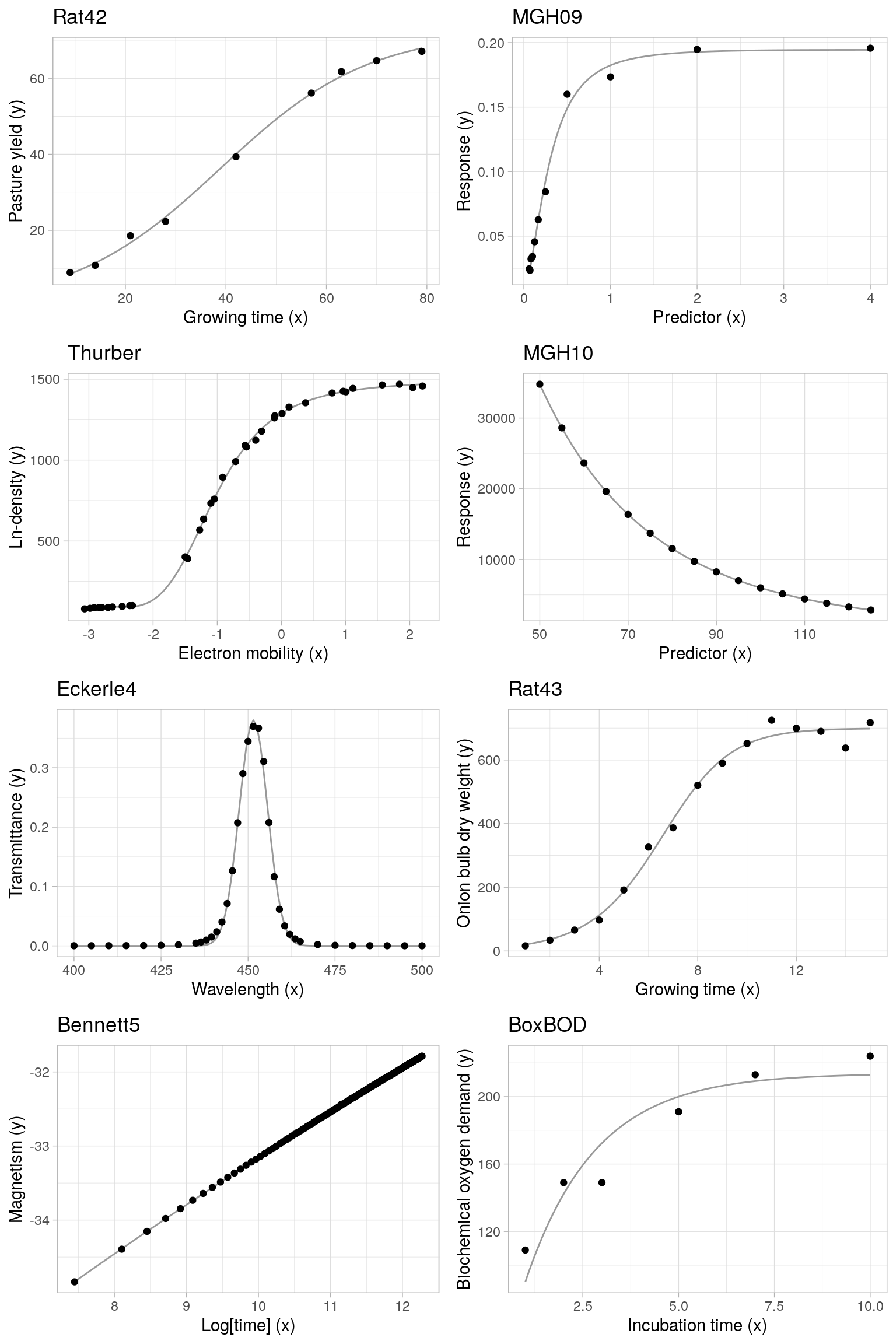
The following plots display all observed datasets, with the (unique) predictor variable on the x-axis and the response variable on the y-axis. The overlayed continuous line corresponds to the regression model evaluated at the certified parameter values.

Algorithms and control parameters

Trust region methods

Convergence of the nonlinear least-squares routines is tested across a grid of algorithms and pre-selected control parameter choices. For the GSL nonlinear least-squares algorithms, all trust region methods available through the gsl_nls() function in the gslnls-package are evaluated, i.e. the algorithm argument in gsl_nls() takes the following values:

"lm", Levenberg-Marquadt algorithm
"lmaccel", Levenberg-Marquadt with geodesic acceleration.
"dogleg", Powell’s Dogleg algorithm
"ddogleg", Double dogleg algorithm
"subspace2D", 2D subspace dogleg generalization.

By default, if the jac argument in the gsl_nls() function is left unspecified, the Jacobian matrix is approximated by (forward) finite differences. Analogously, when geodesic acceleration is used and the fvv argument is left unspecified, the second directional derivatives are approximated by (forward) finite differences. In testing the convergence of the GSL routines, the jac argument is always left unspecified. The Levenberg-Marquadt algorithm with geodesic acceleration is evaluated both with the fvv argument unspecified (denoted by lmaccel) and with fvv = TRUE in which case the second directional derivatives are calculated using algorithmic differentiation (denoted by lmaccel+fvv). To further improve the stability of the lmaccel+fvv method, the acceleration/velocity rejection ratio avmax (see ?gsl_nls_control) is decreased from its default value 0.75 to 0.5, which was found to perform well for the evaluated test problems. For the standard lmaccel method (without algorithmic derivation of fvv), the avmax control parameter is kept at its default value 0.75.

Scaling method

For the control parameters set with gsl_nls_control(), only the scale and solver parameters are varied, see also ?gsl_nls_control. The maximum number of iterations maxiter is increased from the default maxiter = 50 to maxiter = 1e4 in order to remove the maximum number of iterations as a constraining factor, and the default values are used for the remaining control parameters available in gsl_nls_control().

The scale control parameter can take the following values²:

"more", Moré rescaling. This method makes the problem scale-invariant and has been proven effective on a large class of problems.
"levenberg", Levenberg rescaling. This method has also proven effective on a large class of problems, but is not scale-invariant. It may perform better for problems susceptible to parameter evaporation (parameters going to infinity).
"marquadt", Marquadt rescaling. This method is scale-invariant, but it is generally considered inferior to both the Levenberg and Moré strategies.

Solver method

The solver control parameter can take on the following values³:

"qr", QR decomposition of the Jacobian. This method will produce reliable solutions in cases where the Jacobian is rank deficient or near-singular but does require more operations than the Cholesky method.
"cholesky", Cholesky decomposition of the Jacobian. This method is faster than the QR approach, however it is susceptible to numerical instabilities if the Jacobian matrix is rank deficient or near-singular.
"svd", SVD decomposition of the Jacobian. This method will produce the most reliable solutions for ill-conditioned Jacobians but is also the slowest.

Benchmark algorithms

In order to benchmark the performance of the GSL nonlinear least-squares routines against several common R alternatives, each nonlinear regression model is also fitted using the standard nls() function, as well as the nlsLM() function from the minpack.lm-package.

For the nls() function, all three available algorithms are tested, i.e. the algorithm argument is set to respectively:

"default", the default Gauss-Newton algorithm
"plinear", Golub-Pereyra algorithm for partially linear least-squares models
"port", nl2sol algorithm from the Port library

The maximum number of iterations is set to maxiter = 1e4 and the relative convergence tolerance is set to tol = sqrt(.Machine$double.eps) to mimic the control parameters used for the GSL routines.

For the nlsLM() function, there is only a single algorithm (Levenberg-Marquadt), so no choice needs to be made here. The maximum number of iterations is set to maxiter = 1e4 and all other control parameters are kept at their default values.

Rat42 example

As a worked out example, we display the different NLS calls used to fit the Rat42 nonlinear regression model based on gsl_nls(), nls() and nlsLM(). The Rat42 model and data are an example of fitting sigmoidal growth curves taken from (Ratkowsky 1983). The response variable is pasture yield, and the predictor variable is growing times.

Table 2: Rat42 data
y	8.93	10.8	18.59	22.33	39.35	56.11	61.73	64.62	67.08
x	9.00	14.0	21.00	28.00	42.00	57.00	63.00	70.00	79.00

GSL model fit

Similar to nls(), a minimal gsl_nls() function call consists of the model formula, the data and a set of starting values. By default, gsl_nls() uses the Levenberg-Marquadt algorithm (algorithm = "lm") with control parameters scale = "more" and solver = "qr". The starting values $(b_1 = 100, b_2 = 1, b_3 = 0.1)$ are taken from Table 1.

library(NISTnls)    
library(gslnls)     

## gsl Levenberg-Marquadt (more+qr)
rat42_gsl <- gsl_nls(
  fn = y ~ b1 / (1 + exp(b2 - b3 * x)),   ## model
  data = Ratkowsky2,                      ## dataset
  start = c(b1 = 100, b2 = 1, b3 = 0.1)   ## starting values
)

rat42_gsl
#> Nonlinear regression model
#>   model: y ~ b1/(1 + exp(b2 - b3 * x))
#>    data: Ratkowsky2
#>       b1       b2       b3 
#> 72.46224  2.61808  0.06736 
#>  residual sum-of-squares: 8.057
#> 
#> Algorithm: levenberg-marquardt, (scaling: more, solver: qr)
#> 
#> Number of iterations to convergence: 10 
#> Achieved convergence tolerance: 4.619e-14

The gsl_nls() function returns an object that inherits from the class "nls". For this reason, all generic functions available for "nls"-objects are also applicable to objects returned by gsl_nls(). For instance,

## model fit summary
summary(rat42_gsl)
#> 
#> Formula: y ~ b1/(1 + exp(b2 - b3 * x))
#> 
#> Parameters:
#>     Estimate Std. Error t value Pr(>|t|)    
#> b1 72.462238   1.734028   41.79 1.26e-08 ***
#> b2  2.618077   0.088295   29.65 9.76e-08 ***
#> b3  0.067359   0.003447   19.54 1.16e-06 ***
#> ---
#> Signif. codes:  0 '***' 0.001 '**' 0.01 '*' 0.05 '.' 0.1 ' ' 1
#> 
#> Residual standard error: 1.159 on 6 degrees of freedom
#> 
#> Number of iterations to convergence: 10 
#> Achieved convergence tolerance: 4.619e-14

## profile confidence intervals
confint(rat42_gsl)
#>           2.5%       97.5%
#> b1 68.76566669 77.19014998
#> b2  2.41558255  2.84839910
#> b3  0.05947284  0.07600439

Note that the existing predict.nls method is extended to allow for the calculation of asymptotic confidence and prediction intervals, in addition to prediction of the expected response:

predict(rat42_gsl, interval = "prediction", level = 0.95)
#>             fit       lwr      upr
#>  [1,]  8.548006  5.385407 11.71060
#>  [2,] 11.431085  8.235094 14.62708
#>  [3,] 16.727705 13.526235 19.92917
#>  [4,] 23.532240 20.326258 26.73822
#>  [5,] 40.039555 36.612415 43.46669
#>  [6,] 55.963267 52.689429 59.23711
#>  [7,] 60.546511 57.382803 63.71022
#>  [8,] 64.536158 61.311113 67.76120
#>  [9,] 67.913137 64.327402 71.49887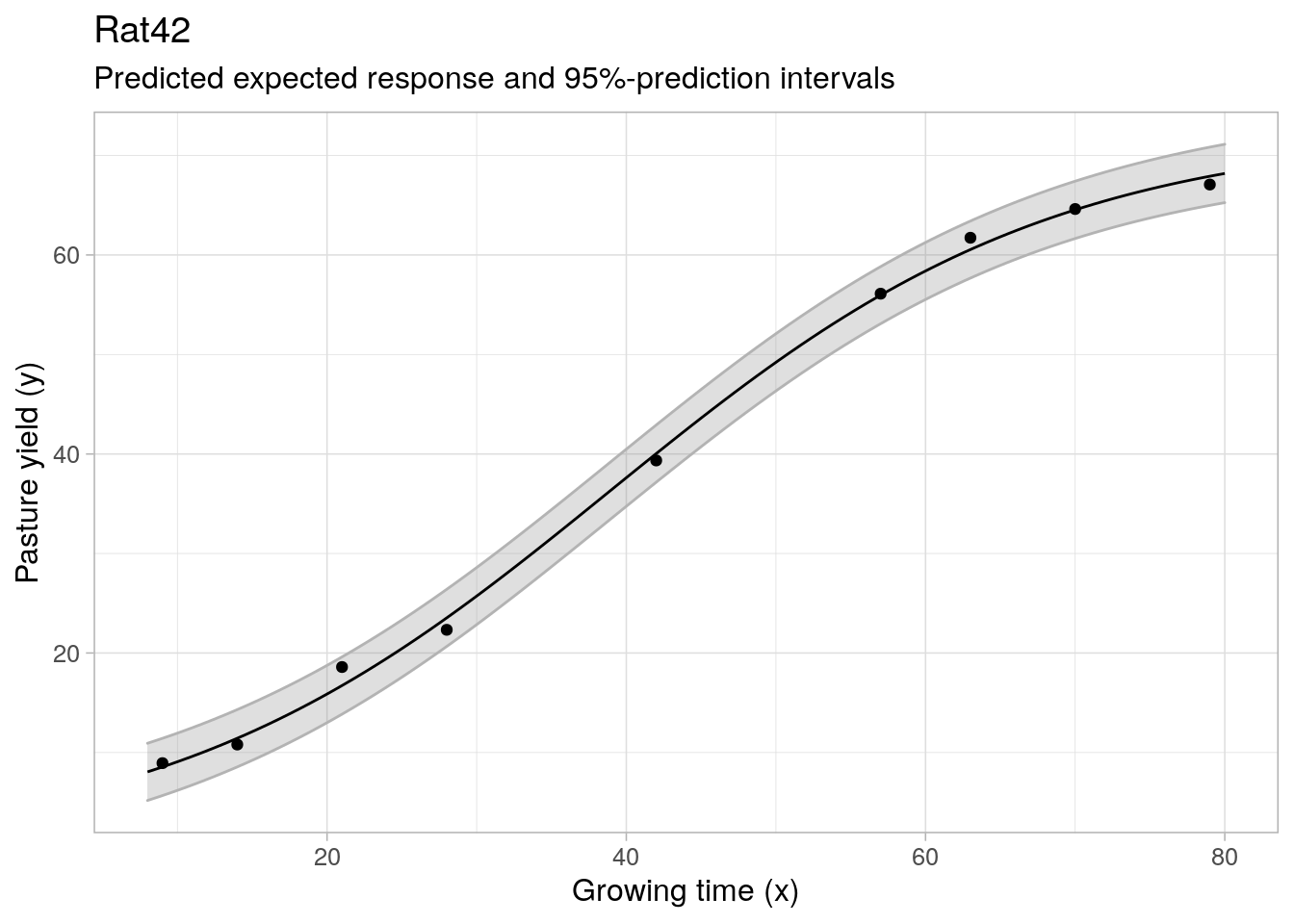

Benchmark NLS fits

As benchmarks to the model fits obtained with gsl_nls(), each test problem is also fitted with calls to nls() and minpack.lm::nlsLM(). For the Rat42 dataset, fitting the regression model with nls() using the default Gauss-Newton algorithm (algorithm = "default") fails to return a valid result:

## nls default
nls(
  formula = y ~ b1 / (1 + exp(b2 - b3 * x)),   ## model
  data = Ratkowsky2,                           ## dataset
  start = c(b1 = 100, b2 = 1, b3 = 0.1)        ## starting values
)
#> Error in nls(formula = y ~ b1/(1 + exp(b2 - b3 * x)), data = Ratkowsky2, : singular gradient

Switching to the Port algorithm (algorithm = "port"), the nls() call does converge to the target least-squares solution:

## nls port
nls(
  formula = y ~ b1 / (1 + exp(b2 - b3 * x)),   ## model
  data = Ratkowsky2,                           ## dataset
  start = c(b1 = 100, b2 = 1, b3 = 0.1),       ## starting values
  algorithm = "port"                           ## algorithm
)
#> Nonlinear regression model
#>   model: y ~ b1/(1 + exp(b2 - b3 * x))
#>    data: Ratkowsky2
#>       b1       b2       b3 
#> 72.46224  2.61808  0.06736 
#>  residual sum-of-squares: 8.057
#> 
#> Algorithm "port", convergence message: relative convergence (4)

And the same is true when using nlsLM() with the default Levenberg-Marquadt algorithm:

## nls LM
minpack.lm::nlsLM(
  formula = y ~ b1 / (1 + exp(b2 - b3 * x)),   ## model
  data = Ratkowsky2,                           ## dataset
  start = c(b1 = 100, b2 = 1, b3 = 0.1),       ## starting values
)
#> Nonlinear regression model
#>   model: y ~ b1/(1 + exp(b2 - b3 * x))
#>    data: Ratkowsky2
#>       b1       b2       b3 
#> 72.46223  2.61808  0.06736 
#>  residual sum-of-squares: 8.057
#> 
#> Number of iterations to convergence: 8 
#> Achieved convergence tolerance: 1.49e-08

The Rat42 model is partially linear in the sense that y ~ b1 * z with z = 1 / (1 + exp(b2 - b3 * x)), which means that the Golub-Pereyra algorithm (algorithm = "plinear") can also be applied in this example. Note that the model formula is updated to exclude the linear parameter b1, and a starting value for this parameter is no longer required.

## nls plinear
nls(
  formula = y ~ 1 / (1 + exp(b2 - b3 * x)),    ## model
  data = Ratkowsky2,                           ## dataset
  start = c(b2 = 1, b3 = 0.1),                 ## starting values
  algorithm = "plinear"                        ## algorithm
)
#> Nonlinear regression model
#>   model: y ~ 1/(1 + exp(b2 - b3 * x))
#>    data: Ratkowsky2
#>       b2       b3     .lin 
#>  2.61808  0.06736 72.46224 
#>  residual sum-of-squares: 8.057
#> 
#> Number of iterations to convergence: 9 
#> Achieved convergence tolerance: 1.119e-06

The p-linear algorithm also converges successfully, with the b1 parameter now labeled as .lin (for linear parameter) in the fitted model coefficients.

Model fit results

Model fit convergence

Below, the convergence status of the evaluated GSL and benchmark NLS routines is displayed for each individual test problem. The obtained convergence results are categorized according to the following status codes:

success; the NLS routine converged successfully and the fitted parameters approximately coincide with the NIST StRD certified values⁴.
false convergence; the NLS routine converged successfully, but the fitted parameters do not coincide with the NIST StRD certified values.
non-zero exit; the NLS routine failed to converge and returns a valid NLS object with a non-zero exit code.
failed; the NLS routine failed to converge and returns an error.

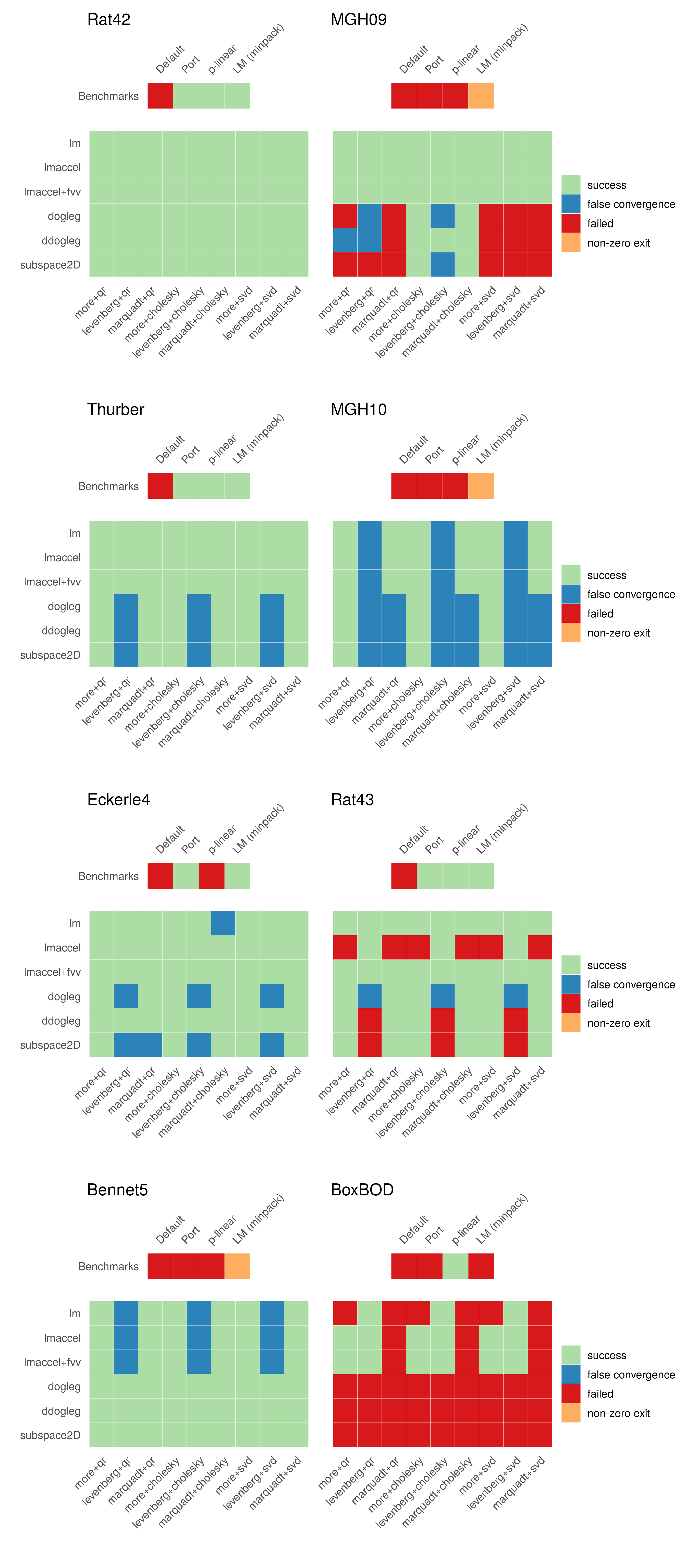
Based on the displayed results, an initial observation is that the default Gauss-Newton algorithm in nls() fails to produce any successful model fit and returns an error for each selected test problem. The Port and (minpack.lm) Levenberg-Marquadt algorithms show roughly similar convergence results, but only successfully converge for half of the evaluated test problems. The p-linear algorithm is somewhat special as it is only applicable for regression models that can be factored into a partially linear model. However, if applicable, the p-linear algorithm can be a powerful alternative as demonstrated by the BoxBOD problem, where most other (general) NLS routines fail to converge. More precisely, the BoxBOD regression model contains only two parameters, and by factoring out the linear parameter, the nonlinear model fit that needs to be optimized by the p-linear algorithm depends only on a single unknown parameter.

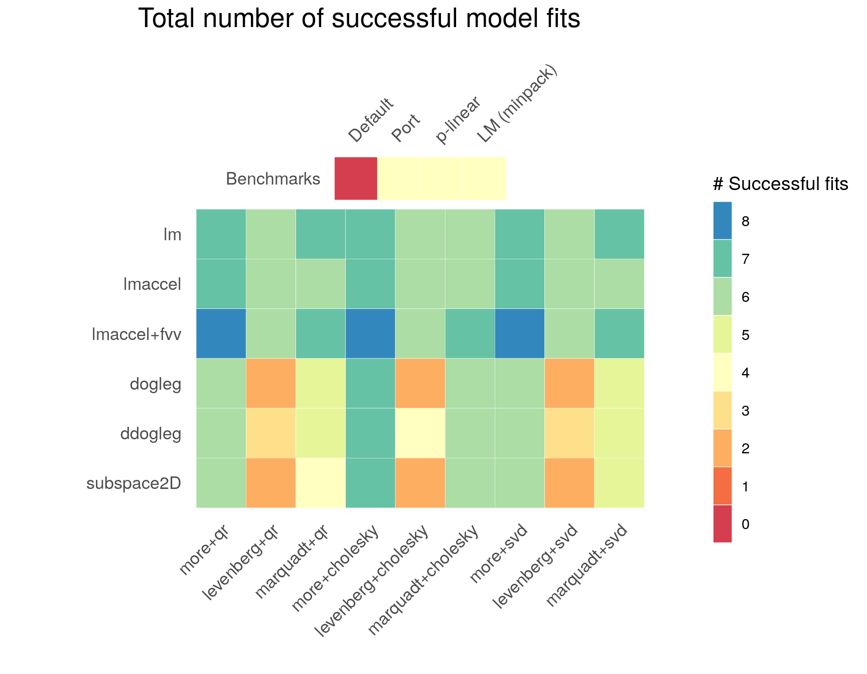
Regarding the GSL routines, for each test problem there exist multiple least-squares algorithms producing a successful model fit. Across test problems and control parameter configurations, the GSL Levenberg-Marquadt algorithms with and without geodesic acceleration (lm, lmaccel, lmaccel+fvv) appear to be the most stable, as also seen in the figure below, which displays the total number of successful model fits across test problems. In comparison to the LM algorithm without geodesic acceleration (lm), the LM algorithm with geodesic acceleration (lmaccel) does not converge for all solver and scaling methods in the Rat43 problem. On the other hand, the LM algorithm with geodesic acceleration is more stable in the BoxBOD problem, where the standard LM algorithm suffers from parameter evaporation. The lmaccel+fvv algorithm shows similar performance to the lmaccel algorithm, and successfully converges across all solver and scaling methods in the Rat43 problem due to the more conservative avmax tuning parameter. In particular, the lmaccel+fvv algorithm with more rescaling is the only routine that converges successfully for all test problems.

Across control parameter configurations, in terms of the scaling method, more rescaling (the default) exhibits the most stable performance, followed by marqaudt rescaling and levenberg rescaling. In the figure below, this is seen most prominently for the different variations of the Dogleg algorithm (dogleg, ddogleg, subspace2D) and somewhat less for the Levenberg-Marquadt algorithms. The chosen solver method seems to be less impactful for the evaluated test problems, with the cholesky solver method producing slightly more robust results than the qr and svd solver methods respectively.

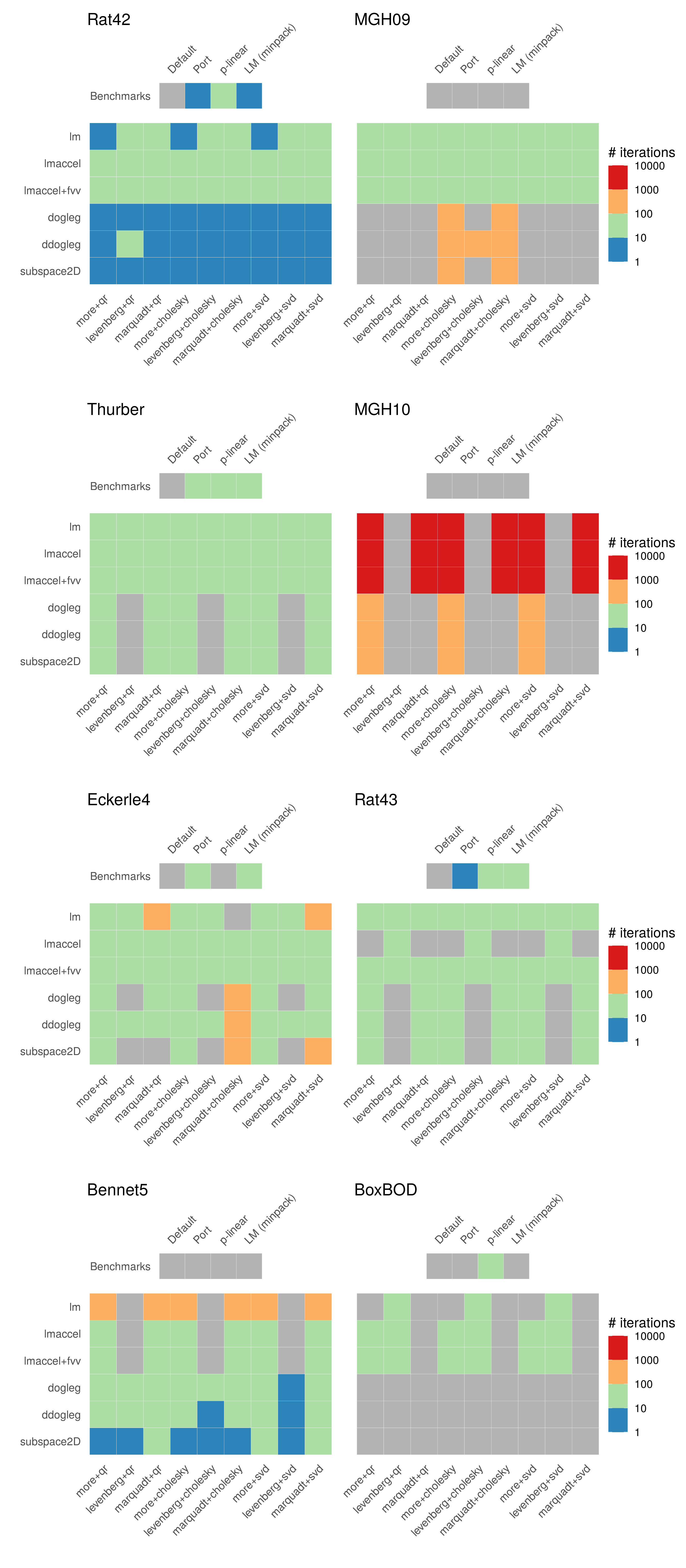
Iterations to convergence

As supplementary information, we also display the required number of iterations to reach convergence for each successfully converged NLS routine. In case of a successful model fit, the Port algorithm requires only a small number of iterations to reach convergence. The number of iterations required by the minpack.lm Levenberg-Marquadt algorithm and GSL Levenberg-Marquadt algorithm(s) is of the same order of magnitude. Among the GSL routines, except for the MGH09 problem, the general tendency is that the Dogleg-based algorithms (dogleg, ddogleg, subspace2D) require less iterations than the LM-based algorithms. This is illustrated most clearly by the Rat42 and Bennet5 plots.

Conclusion

Based on a small collection of NIST StRD test problems, this post benchmarks the convergence properties of a number of GSL nonlinear least squares routines as well as several standard NLS algorithms that are in common use. For the tested nonlinear regression problems, the GSL algorithms show at least comparable –and often better– optimization performance than the included benchmark algorithms, using mostly standard choices and default values for the GSL trust region method control parameters. As such, the GSL trust region methods provide a useful supplement to the existing suite of nonlinear least squares fitting algorithms available in R, in particular when adequate starting values are difficult to come by and more stable optimization routines (than provided by R’s standard methods) are required.

Session Info

sessionInfo()
#> R version 4.1.1 (2021-08-10)
#> Platform: x86_64-pc-linux-gnu (64-bit)
#> Running under: Ubuntu 18.04.6 LTS
#> 
#> Matrix products: default
#> BLAS:   /usr/lib/x86_64-linux-gnu/blas/libblas.so.3.7.1
#> LAPACK: /usr/lib/x86_64-linux-gnu/lapack/liblapack.so.3.7.1
#> 
#> locale:
#>  [1] LC_CTYPE=en_US.UTF-8       LC_NUMERIC=C              
#>  [3] LC_TIME=en_US.UTF-8        LC_COLLATE=en_US.UTF-8    
#>  [5] LC_MONETARY=en_US.UTF-8    LC_MESSAGES=en_US.UTF-8   
#>  [7] LC_PAPER=en_US.UTF-8       LC_NAME=C                 
#>  [9] LC_ADDRESS=C               LC_TELEPHONE=C            
#> [11] LC_MEASUREMENT=en_US.UTF-8 LC_IDENTIFICATION=C       
#> 
#> attached base packages:
#> [1] stats     graphics  grDevices utils     datasets  methods   base     
#> 
#> other attached packages:
#> [1] gslnls_1.0.3      NISTnls_0.9-13    patchwork_1.1.1   ggplot2_3.3.5    
#> [5] data.table_1.14.2 kableExtra_1.3.4  knitr_1.36       
#> 
#> loaded via a namespace (and not attached):
#>  [1] minpack.lm_1.2-1   tidyselect_1.1.1   xfun_0.26          bslib_0.3.1       
#>  [5] purrr_0.3.4        colorspace_2.0-2   vctrs_0.3.8        generics_0.1.0    
#>  [9] htmltools_0.5.2    viridisLite_0.4.0  yaml_2.2.1         utf8_1.2.2        
#> [13] rlang_0.4.11       jquerylib_0.1.4    pillar_1.6.3       glue_1.4.2        
#> [17] withr_2.4.2        RColorBrewer_1.1-2 lifecycle_1.0.1    stringr_1.4.0     
#> [21] munsell_0.5.0      blogdown_1.5       gtable_0.3.0       rvest_1.0.1       
#> [25] evaluate_0.14      labeling_0.4.2     fastmap_1.1.0      fansi_0.5.0       
#> [29] highr_0.9          scales_1.1.1       webshot_0.5.2      jsonlite_1.7.2    
#> [33] farver_2.1.0       systemfonts_1.0.2  gridExtra_2.3      digest_0.6.28     
#> [37] stringi_1.7.4      bookdown_0.24      dplyr_1.0.7        grid_4.1.1        
#> [41] tools_4.1.1        magrittr_2.0.1     sass_0.4.0         tibble_3.1.5      
#> [45] crayon_1.4.1       pkgconfig_2.0.3    MASS_7.3-54        ellipsis_0.3.2    
#> [49] xml2_1.3.2         rmarkdown_2.11     svglite_2.0.0      httr_1.4.2        
#> [53] rstudioapi_0.13    R6_2.5.1           compiler_4.1.1

References

Bennett, L., L. Swartzendruber, and H. Brown. 1994. “Superconductivity Magnetization Modeling.” National Institute of Standards and Technology (NIST), US Department of Commerce, USA.

Box, G. P., W. H. Hunter, S. Hunter, et al. 1978. Statistics for Experimenters. New York: Wiley.

Eckerle, K. 1979. “Circular Interference Transmittance Study.” National Institute of Standards and Technology (NIST), US Department of Commerce, USA 13.

Galassi, M., J. Davies, J. Theiler, B. Gough, G. Jungman, M. Booth, and F. Rossi. 2009. GNU Scientific Library Reference Manual. 3rd ed. Network Theory Limited. https://www.gnu.org/software/gsl/.

Kowalik, J. S., and M. R. Osborne. 1978. Methods for Unconstrained Optimization Problems. New York: Elsevier.

Meyer, R. R. 1970. “Theoretical and Computational Aspects of Nonlinear Regression.” In Nonlinear Programming, 465–86. New York: Elsevier.

Moré, J. J., B. S. Garbow, and K. E. Hillstrom. 1981. “Testing Unconstrained Optimization Software.” ACM Transactions on Mathematical Software (TOMS) 7 (1): 17–41.

Ratkowsky, D. 1983. Nonlinear Regression Modelling. New York: Marcel Dekker.

Thurber, R. 1979. “Semiconductor Electron Mobility Modeling.” National Institute of Standards and Technology (NIST), US Department of Commerce, USA.

https://cran.r-project.org/web/packages/NISTnls/index.html ↩︎
https://www.gnu.org/software/gsl/doc/html/nls.html#c.gsl_multifit_nlinear_scale ↩︎
https://www.gnu.org/software/gsl/doc/html/nls.html#c.gsl_multifit_nlinear_solver ↩︎
Here, the maximum relative deviation of the fitted values with respect to the certified values is within a small tolerance range $\epsilon$.↩︎

GSL gslnls R Nonlinear least squares GNU Scientific Library NIST StRD