Automatic differentiation in R with Stan Math
With applications to nonlinear least squares regression
Introduction
Automatic differentiation
Automatic differentiation (AD) refers to the automatic/algorithmic calculation of derivatives of a function defined as a computer program by repeated application of the chain rule. Automatic differentiation plays an important role in many statistical computing problems, such as gradient-based optimization of large-scale models, where gradient calculation by means of numeric differentiation (i.e. finite-differencing) is not sufficiently accurate or too slow and manual (or symbolic) differentiation of the function as a mathematical expression is unfeasible. Given its importance, many AD tools have been developed for use in different scientific programming languages, and a large curated list of existing AD libraries can be found at autodiff.org. In this post, we focus on the use of the C++ Stan Math library, which contains forward- and reverse-mode AD implementations aimed at probability, linear algebra and ODE applications and is used as the underlying library to perform automatic differentiation in Stan. See (Carpenter et al. 2015) for a comprehensive overview of the Stan Math library and instructions on its usage.
This post requires some working knowledge of Stan and Rcpp in order to write model functions using Stan Math in C++ and expose these functions to R.
Symbolic differentiation in R
Base R
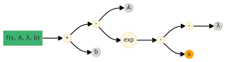
Simple composite expressions and formulas can be derived efficiently using stats::D() for derivatives with respect to a single parameter, or the more general stats::deriv() for (partial) derivatives with respect to multiple parameters. The deriv() function calculates derivatives symbolically by chaining the derivatives of each individual operator/function in the expression tree through repeated application of the chain rule. To illustrate, consider the exponential model:
\[ f(x, A, \lambda, b) \ = \ A \exp(-\lambda x) + b \]
with independent variable \(x\) and parameters \(A\), \(\lambda\) and \(b\). Deriving this function manually gives the following gradient:
\[
\nabla f \ = \ \left[ \frac{\partial f}{\partial A}, \frac{\partial f}{\partial \lambda}, \frac{\partial f}{\partial b} \right] \ = \ \left[ \exp(-\lambda x), -A \exp(-\lambda x) x, 1 \right]
\]
Using the deriv() function, we can obtain the same gradient algorithmically:
## gradient function
(fdot <- deriv(~A * exp(-lam * x) + b, namevec = c("A", "lam", "b"), function.arg = c("x", "A", "lam", "b")))
#> function (x, A, lam, b)
#> {
#>     .expr3 <- exp(-lam * x)
#>     .value <- A * .expr3 + b
#>     .grad <- array(0, c(length(.value), 3L), list(NULL, c("A",
#>         "lam", "b")))
#>     .grad[, "A"] <- .expr3
#>     .grad[, "lam"] <- -(A * (.expr3 * x))
#>     .grad[, "b"] <- 1
#>     attr(.value, "gradient") <- .grad
#>     .value
#> }
Since we specified the function.arg argument, deriv() returns a function –instead of an expression– that can be used directly to evaluate both the function values and the gradient (or Jacobian) for different values of the independent variable and parameters. Inspecting the body of the returned function, we see that the expression in the "gradient" attribute corresponds exactly to the manually derived gradient.
## evaluate function + jacobian
fdot(x = (1:10) / 10, A = 5, lam = 1.5, b = 1)
#>  [1] 5.303540 4.704091 4.188141 3.744058 3.361833 3.032848 2.749689 2.505971
#>  [9] 2.296201 2.115651
#> attr(,"gradient")
#>               A        lam b
#>  [1,] 0.8607080 -0.4303540 1
#>  [2,] 0.7408182 -0.7408182 1
#>  [3,] 0.6376282 -0.9564422 1
#>  [4,] 0.5488116 -1.0976233 1
#>  [5,] 0.4723666 -1.1809164 1
#>  [6,] 0.4065697 -1.2197090 1
#>  [7,] 0.3499377 -1.2247821 1
#>  [8,] 0.3011942 -1.2047768 1
#>  [9,] 0.2592403 -1.1665812 1
#> [10,] 0.2231302 -1.1156508 1
Note that the returned matrix in the "gradient" attribute corresponds to the Jacobian matrix, with each row of the matrix containing the partial derivatives with respect to one value \(x_i\) of the independent variable.
The deriv() and D() functions are useful for the derivation of composite expressions of standard arithmetic operators and functions, as commonly used for instance for the specification of simple nonlinear models, (see ?deriv for the complete list of operators and functions recognized by deriv()). As such, the scope of these functions is rather limited compared to general AD tools, which can handle function definitions that include control flow statements, concatenations, reductions, matrix algebra, etc.
Below are some example expressions that cannot be differentiated with deriv():
## reductions
deriv(~sum((y - x * theta)^2), namevec = "theta")
#> Error in deriv.formula(~sum((y - x * theta)^2), namevec = "theta"): Function 'sum' is not in the derivatives table

## concatenation/matrix product
deriv(~X %*% c(theta1, theta2, theta3), namevec = "theta1")
#> Error in deriv.formula(~X %*% c(theta1, theta2, theta3), namevec = "theta1"): Function '`%*%`' is not in the derivatives table

## user-defined function
f <- function(x, y) x^2 + y^2
deriv(~f(x, y), namevec = "x")
#> Error in deriv.formula(~f(x, y), namevec = "x"): Function 'f' is not in the derivatives table
The Deriv-package
The Deriv() function in the Deriv-package provides a much more flexible symbolic differentiation interface, which also allows custom functions to be added to the derivative table. Using Deriv(), we can produce derivatives in each of the problematic cases above:
library(Deriv)

## reductions
Deriv(~sum((y - x * theta)^2), x = "theta")
#> sum(-(2 * (x * (y - theta * x))))

## concatenation/matrix product
Deriv(~X %*% c(theta1, theta2, theta3), x = "theta1")
#> X %*% c(1, 0, 0)

## user-defined function
f <- function(x, y) x^2 + y^2
Deriv(~f(x, y), x = "x")
#> 2 * x
Limits of symbolic differentiation with Deriv
Even though the Deriv() function is quite powerful in terms of symbolic differentiation, its scope remains limited to
straightforward expression graphs, with a small number of parameters. For example, consider deriving a polynomial function of degree 10 given by:
\[
f(\boldsymbol{\theta}) \ = \ \sum_{k = 0}^{10} \theta_k x^k
\]
with parameters \(\boldsymbol{\theta} = (\theta_0, \ldots, \theta_{10})\). Using the Deriv() function, derivative calculation with respect to \(\boldsymbol{\theta}\) becomes quite cumbersome, as the complete polynomial needs to be written out as a function of the individual parameters:
fpoly <- function(theta0, theta1, theta2, theta3, theta4, theta5, theta6, theta7, theta8, theta9, theta10, x) {
  sum(c(theta0, theta1, theta2, theta3, theta4, theta5, theta6, theta7, theta8, theta9, theta10) * c(1, x, x^2, x^3, x^4, x^5, x^6, x^7, x^8, x^9, x^10))
}

Deriv(~fpoly(theta0, theta1, theta2, theta3, theta4, theta5, theta6, theta7, theta8, theta9, theta10, x),
      x = c("theta0", "theta1", "theta2", "theta3", "theta4", "theta5", "theta6", "theta7", "theta8", "theta9", "theta10"))
#> {
#>     .e1 <- c(0, 0, 0, 0, 0, 0, 0, 0, 0, 0, 0) * c(theta0, theta1,
#>         theta2, theta3, theta4, theta5, theta6, theta7, theta8,
#>         theta9, theta10)
#>     .e2 <- c(1, x, x^2, x^3, x^4, x^5, x^6, x^7, x^8, x^9, x^10)
#>     c(theta0 = sum(.e1 + c(1, 0, 0, 0, 0, 0, 0, 0, 0, 0, 0) *
#>         .e2), theta1 = sum(.e1 + c(0, 1, 0, 0, 0, 0, 0, 0, 0,
#>     0, 0) * .e2), theta2 = sum(.e1 + c(0, 0, 1, 0, 0, 0, 0, 0,
#>     0, 0, 0) * .e2), theta3 = sum(.e1 + c(0, 0, 0, 1, 0, 0, 0,
#>     0, 0, 0, 0) * .e2), theta4 = sum(.e1 + c(0, 0, 0, 0, 1, 0,
#>     0, 0, 0, 0, 0) * .e2), theta5 = sum(.e1 + c(0, 0, 0, 0, 0,
#>     1, 0, 0, 0, 0, 0) * .e2), theta6 = sum(.e1 + c(0, 0, 0, 0,
#>     0, 0, 1, 0, 0, 0, 0) * .e2), theta7 = sum(.e1 + c(0, 0, 0,
#>     0, 0, 0, 0, 1, 0, 0, 0) * .e2), theta8 = sum(.e1 + c(0, 0,
#>     0, 0, 0, 0, 0, 0, 1, 0, 0) * .e2), theta9 = sum(.e1 + c(0,
#>     0, 0, 0, 0, 0, 0, 0, 0, 1, 0) * .e2), theta10 = sum(.e1 +
#>         c(0, 0, 0, 0, 0, 0, 0, 0, 0, 0, 1) * .e2))
#> }
Note also the over-complicated expressions for the calculated derivatives. Preferably, we would write the polynomial function along the lines of:
fpoly <- function(theta, x) {
  y <- theta[1]
  for(k in 1:10) {
    y <- y + theta[k + 1] * x^k
  }
  return(y)
}
and differentiate the polynomial with respect to all elements of \(\boldsymbol{\theta}\). This is a complex symbolic differentation task, but is a natural use-case for (forward- or reverse-mode) automatic differentiation.
Prerequisites
The Stan Math C++ header files are contained within the StanHeaders-package and in order to use the Stan Math library, it suffices to install the StanHeaders package in R. At the moment of writing, the CRAN version of StanHeaders is several versions behind the latest Stan release. A more recent version of StanHeaders is available from the package repository at https://mc-stan.org/r-packages/:
## install dependencies
install.packages(c("BH", "Rcpp", "RcppEigen", "RcppParallel"))
install.packages("StanHeaders", repos = c("https://mc-stan.org/r-packages/", getOption("repos")))
In this post, we compile C++ files making use of Stan Math with Rcpp::sourceCpp(). In order to instruct the C++ compiler about the locations of the header files and shared libraries (in addition to setting some compiler flags), we can execute the following lines of code1 once at the start of the R session:
## update PKG_CXXFLAGS and PKG_LIBS
Sys.setenv(PKG_CXXFLAGS = StanHeaders:::CxxFlags(as_character = TRUE))
SH <- system.file(ifelse(.Platform$OS.type == "windows", "libs", "lib"), .Platform$r_arch, package = "StanHeaders", mustWork = TRUE)
Sys.setenv(PKG_LIBS = paste0(StanHeaders:::LdFlags(as_character = TRUE), " -L", shQuote(SH), " -lStanHeaders"))
Sys.getenv("PKG_CXXFLAGS")
#> [1] "-I'/home/jchau/R/x86_64-pc-linux-gnu-library/4.1/RcppParallel/include' -D_REENTRANT -DSTAN_THREADS"
Sys.getenv("PKG_LIBS")
#> [1] "-L'/home/jchau/R/x86_64-pc-linux-gnu-library/4.1/RcppParallel/lib/' -Wl,-rpath,'/home/jchau/R/x86_64-pc-linux-gnu-library/4.1/RcppParallel/lib/' -ltbb -ltbbmalloc -L'/home/jchau/R/x86_64-pc-linux-gnu-library/4.1/StanHeaders/lib/' -lStanHeaders"The above code can also be included in e.g. ~/.Rprofile, so that it is executed automatically when starting a new R session. The above steps are combined in the following dockerfile, which sets up an image based on rocker/r-ver:4.1 capable of compiling C++ files with Rcpp that use Stan Math.
# R-base image
FROM rocker/r-ver:4.1
# install dependencies
RUN R -e 'install.packages(c("BH", "Rcpp", "RcppEigen", "RcppParallel"), repos = "https://cran.r-project.org/")'
# install StanHeaders
RUN R -e 'install.packages("StanHeaders", repos = "https://mc-stan.org/r-packages/")'
# generate .Rprofile
RUN R -e 'file.create("/root/.Rprofile"); \
cat("Sys.setenv(PKG_CXXFLAGS = \"", StanHeaders:::CxxFlags(as_character = TRUE), "\")\n", file = "/root/.Rprofile"); \
cat("Sys.setenv(PKG_LIBS = \"", paste0(StanHeaders:::LdFlags(as_character = TRUE), " -L", \
shQuote(system.file("lib", package = "StanHeaders")), " -lStanHeaders"), "\")\n", file = "/root/.Rprofile", append = TRUE)'
# launch R
CMD ["R"]
R-packages interfacing Stan Math
If the intention is to use Stan Math in another R-package then the DESCRIPTION file of the package should include:
LinkingTo: StanHeaders (>= 2.21.0), RcppParallel (>= 5.0.1)
SystemRequirements: GNU make
and the following lines can be added to src/Makevars and src/Makevars.win:
CXX_STD = CXX14
PKG_CXXFLAGS = $(shell "$(R_HOME)/bin$(R_ARCH_BIN)/Rscript" -e "RcppParallel::CxxFlags()") $(shell "$(R_HOME)/bin$(R_ARCH_BIN)/Rscript" -e "StanHeaders:::CxxFlags()")
PKG_LIBS = $(shell "$(R_HOME)/bin$(R_ARCH_BIN)/Rscript" -e "RcppParallel::RcppParallelLibs()") $(shell "$(R_HOME)/bin$(R_ARCH_BIN)/Rscript" -e "StanHeaders:::LdFlags()")Remark: Instead of manually adding these entries, consider using the rstantools-package, which automatically generates the necessary file contents as well as the appropriate folder structure for an R-package interfacing with Stan Math (or Stan in general).
Examples
Example 1: Polynomial function
As a first minimal example, consider again the polynomial function of degree 10 defined above, but now with the gradient calculated by means of automatic differentiation instead of symbolic differentiation. The automatic differentiation is performed by the stan::math::gradient() functional, which takes the function to derive as an argument in the form of a functor or a lambda expression. In particular, the polynomial function can be encoded as a lambda expression as follows:
// polynomial function
[x](auto theta) {
  auto y = theta[0];
  for(int k = 1; k < theta.size(); k++) {
    y += theta[k] * std::pow(x, k);
  }
  return y;
}
Here, the [x] clause captures the x variable by value from the surrounding scope. If x is prefixed by an &, then the variable x is accessed by reference instead. The parameter list (auto theta) defines the parameters with respect to which the (partial) derivatives are evaluated, in this case all the elements of the vector theta. The lambda body contains the definition of the function to derive, which is the C++ equivalent of the polynomial definition at the end of the first section.
The remaining arguments passed to stan::math::gradient() are respectively; an (Eigen) array of parameter values at which to evaluate the gradient, a scalar to hold the value of the evaluated function, and an (Eigen) array to hold the values of the evaluated gradient.
In order to expose the gradient functional to R, we write a minimal Rcpp wrapper function that takes a scalar value x and a numeric vector theta as arguments, and returns the evaluated gradient at x and theta as a numeric vector of the same length as theta. Inserting the necessary Rcpp::depends() and #include statements, analogous to the Using the Stan Math C++ Library vignette, we compile the following C++ code with Rcpp::sourceCpp():
// [[Rcpp::depends(BH)]]
// [[Rcpp::depends(RcppEigen)]]
// [[Rcpp::depends(RcppParallel)]]
// [[Rcpp::depends(StanHeaders)]]
#include <stan/math.hpp>  // pulls in everything from rev/ and prim/
#include <Rcpp.h>
#include <RcppEigen.h>

// [[Rcpp::plugins(cpp14)]]

// [[Rcpp::export]]
auto grad_poly(double x, Eigen::VectorXd theta)
{
  // declarations
  double fx;
  Eigen::VectorXd grad_fx;

  // gradient calculation
  stan::math::gradient([x](auto theta) {
    // polynomial function
    auto y = theta[0];
    for(int k = 1; k < theta.size(); k++) {
      y += theta[k] * std::pow(x, k);
    }
    return y;
  }, theta, fx, grad_fx);

  // evaluated gradient
  return grad_fx;
}Remark: By default #include <stan/math.hpp> includes the reverse-mode implementation of stan::math::gradient() based on <stan/math/rev.hpp>. To use the forward-mode implementation of stan::math::gradient(), we can first include <stan/math/fwd.hpp> before including <stan/math.hpp> (if also necessary).
The compiled function grad_poly() can now be called in R to evaluate the reverse-mode gradient of the polynomial function at any given value of x and theta2:
## evaluated gradient
grad_poly(x = 0.5, theta = rep(1, 11))
#>  [1] 1.0000000000 0.5000000000 0.2500000000 0.1250000000 0.0625000000
#>  [6] 0.0312500000 0.0156250000 0.0078125000 0.0039062500 0.0019531250
#> [11] 0.0009765625
and the result corresponds exactly to the evaluated gradient obtained by deriving the polynomial function analytically:
## analytic gradient
x <- 0.5
x^(0:10)
#>  [1] 1.0000000000 0.5000000000 0.2500000000 0.1250000000 0.0625000000
#>  [6] 0.0312500000 0.0156250000 0.0078125000 0.0039062500 0.0019531250
#> [11] 0.0009765625
Example 2: Exponential model
As a second example, we consider calculation of the Jacobian for the exponential model defined above. In order to calculate the (reverse-mode) Jacobian matrix, we use the stan::math::jacobian() functional, which takes the function to derive as an argument in the form of a functor or lambda expression analogous to stan::math::gradient(). The other arguments passed to stan::math::jacobian() are respectively; an (Eigen) array of parameter values at which to evaluate the Jacobian, an (Eigen) array to hold the values of the evaluated function, and an (Eigen) matrix to hold the values of the evaluated Jacobian.
Similar to the previous example, we define a C++ wrapper function, which in the current example takes as inputs the vector-valued independent variable x and the vector of parameter values theta. The wrapper function returns both the function value and the Jacobian in the same format as deriv() by including the Jacobian matrix in the "gradient" attribute of the evaluated function value. The following C++ code is compiled with Rcpp::sourceCpp():
// [[Rcpp::depends(BH)]]
// [[Rcpp::depends(RcppEigen)]]
// [[Rcpp::depends(RcppParallel)]]
// [[Rcpp::depends(StanHeaders)]]
#include <stan/math.hpp>
#include <Rcpp.h>
#include <RcppEigen.h>

// [[Rcpp::plugins(cpp14)]]

using namespace Rcpp;

// [[Rcpp::export]]
auto fjac_exp(Eigen::VectorXd x, Eigen::VectorXd theta)
{
  // declarations
  Eigen::VectorXd fx;
  Eigen::MatrixXd jac_fx;

  // response and jacobian
  stan::math::jacobian([&x](auto theta) {
    // exponential model
    return stan::math::add(theta(0) * stan::math::exp(-theta(1) * x), theta(2));
  }, theta, fx, jac_fx);

  // reformat returned result
  NumericVector fx1 = wrap(fx);
  NumericMatrix jac_fx1 = wrap(jac_fx);
  colnames(jac_fx1) = CharacterVector({"A", "lam", "b"});
  fx1.attr("gradient") = jac_fx1;

  return fx1;
}
The exponential model function is expressed concisely using the vectorized functions stan::math::add() and stan::math::exp(). Also, the return type is deduced automatically in the lambda expression and does not need to be specified explicitly. After compilation, we can evaluate the Jacobian of the exponential model in R by calling the jac_exp() function with input values for x and theta:
## evaluated jacobian
fjac_exp(x = (1:10) / 10, theta = c(5, 1.5, 1))
#>  [1] 5.303540 4.704091 4.188141 3.744058 3.361833 3.032848 2.749689 2.505971
#>  [9] 2.296201 2.115651
#> attr(,"gradient")
#>               A        lam b
#>  [1,] 0.8607080 -0.4303540 1
#>  [2,] 0.7408182 -0.7408182 1
#>  [3,] 0.6376282 -0.9564422 1
#>  [4,] 0.5488116 -1.0976233 1
#>  [5,] 0.4723666 -1.1809164 1
#>  [6,] 0.4065697 -1.2197090 1
#>  [7,] 0.3499377 -1.2247821 1
#>  [8,] 0.3011942 -1.2047768 1
#>  [9,] 0.2592403 -1.1665812 1
#> [10,] 0.2231302 -1.1156508 1
and we can verify that the returned values are equal to the results obtained by symbolic derivation with deriv():
## test for equivalence
all.equal(
  fjac_exp(x = (1:10) / 10, theta = c(5, 1.5, 1)),
  fdot(x = (1:10) / 10, A = 5, lam = 1.5, b = 1)
)
#> [1] TRUE
Nonlinear least squares
Simulated data
As an application of the Jacobian calculations, we consider automatic differentiation in the context of gradient-based nonlinear least squares optimization. Let \(y_1,\ldots,y_n\) be a set of noisy observations generated from the exponential model function \(f(x, A, \lambda, b) = A \exp(-\lambda x) + b\) corrupted by i.i.d. Gaussian noise:
\[ \left\{ \begin{aligned} y_i &\ = \ f(x_i, A, \lambda, b) + \epsilon_i, \\ \epsilon_i &\ = \ N(0, \sigma^2), \quad \quad \quad \quad \quad i = 1, \ldots, n \end{aligned} \right. \]
The independent variables \(\boldsymbol{x} = (x_1,\ldots,x_n)\) are assumed to be known and the parameters \(\boldsymbol{\theta} = (A, \lambda, b)'\) are the estimation targets. The following code generates \(n = 50\) noisy observations with model parameters \(A = 5\), \(\lambda = 1.5\), \(b = 1\) and noise standard deviation \(\sigma = 0.25\):
set.seed(1)
n <- 50
x <- (seq_len(n) - 1) * 3 / (n - 1)
f <- function(x, A, lam, b) A * exp(-lam * x) + b
y <- f(x, A = 5, lam = 1.5, b = 1) + rnorm(n, sd = 0.25)
Model fit
To obtain parameter estimates based on the generated data, we fit the exponential model by means of nonlinear least squares regression with the gsl_nls() function in the gslnls-package. The gslnls-package provides R bindings to gradient-based nonlinear least squares optimization with the GNU Scientific Library (GSL). By default, the gsl_nls() function uses numeric differentiation to evaluate the Jacobian matrix at each step in the nonlinear least squares routine. For simple model formulas, the Jacobian matrix can also be obtained through symbolic differentiation with deriv(). Using the Stan Math library, we acquire a third automated procedure to evaluate the Jacobian matrix, which is by means of automatic differentiation:
library(gslnls)

## symbolic differentiation
gsl_nls(
  fn = y ~ A * exp(-lam * x) + b,     ## model formula
  data = data.frame(x = x, y = y),    ## model fit data
  start = c(A = 0, lam = 0, b = 0),   ## starting values
  algorithm = "lm",                   ## levenberg-marquadt
  jac = TRUE                          ## symbolic derivation
)
#> Nonlinear regression model
#>   model: y ~ A * exp(-lam * x) + b
#>    data: data.frame(x = x, y = y)
#>      A    lam      b
#> 4.9905 1.4564 0.9968
#>  residual sum-of-squares: 2.104
#>
#> Algorithm: multifit/levenberg-marquardt, (scaling: more, solver: qr)
#>
#> Number of iterations to convergence: 8
#> Achieved convergence tolerance: 9.496e-11

## automatic differentiation
gsl_nls(
  fn = y ~ fjac_exp(x, c(A, lam, b)),
  data = data.frame(x = x, y = y),
  start = c(A = 0, lam = 0, b = 0),
  algorithm = "lm"
)
#> Nonlinear regression model
#>   model: y ~ fjac_exp(x, c(A, lam, b))
#>    data: data.frame(x = x, y = y)
#>      A    lam      b
#> 4.9905 1.4564 0.9968
#>  residual sum-of-squares: 2.104
#>
#> Algorithm: multifit/levenberg-marquardt, (scaling: more, solver: qr)
#>
#> Number of iterations to convergence: 8
#> Achieved convergence tolerance: 9.496e-11
In this example, gradient calculation by means of automatic differentiation is unnecessary, as the simple exponential model formula can be derived symbolically requiring much less effort to set up. The next example considers a slightly more complex nonlinear regression problem, where symbolic differentiation is no longer applicable, but automatic differentiation can be used instead.
Example 3: Watson function
The Watson function is a common test problem in nonlinear least squares optimization and is defined as Problem 20 in (Moré, Garbow, and Hillstrom 1981). Consider observations \((f_1,\ldots,f_n)\) generated from the following model:
\[ \begin{cases} f_i & = & \sum_{j = 2}^p (j - 1) \ \theta_j t_i^{j-2} - \left( \sum_{j = 1}^p \theta_j t_i^{j-1}\right) - 1, \quad \quad 1 \leq i \leq n - 2, \\ f_{n-1} & = & \theta_1, \\ f_n & = & \theta_2 - \theta_1^2 - 1 \end{cases} \]
with parameters \(\boldsymbol{\theta} = (\theta_1,\ldots,\theta_p)\) and independent variables \(t_i = i / n\). Similar to the model definition in (Moré, Garbow, and Hillstrom 1981), we set the number of parameters to \(p = 6\) and the number of observations to \(n = 31\). The Watson function is encoded in R as follows:
f_watson <- function(theta) {
  n <- 31
  p <- length(theta)
  ti <- (1:(n - 2)) / (n - 2)
  tj <- rep(1, n - 2)
  sum1 <- rep(theta[1], n - 2)
  sum2 <- rep(0, n - 2)
  for(j in 2:p) {
    sum2 <- sum2 + (j - 1) * theta[j] * tj
    tj <- tj * ti
    sum1 <- sum1 + theta[j] * tj
  }
  c(sum2 - sum1^2 - 1, theta[1], theta[2] - theta[1]^2 - 1)
}
The goal in this example is to find the parameter estimates \(\hat{\boldsymbol{\theta}} = (\hat{\theta}_1, \ldots, \hat{\theta}_6)\) that minimize the sum-of-squares (i.e. the least squares estimates):
\[ \hat{\boldsymbol{\theta}} \ = \ \arg\min_\theta \sum_{i = 1}^n f_i^2 \]
which can be solved using the gsl_nls() function (or e.g. minpack.lm::nls.lm()) by passing the nonlinear model as a function and setting the response vector to zero:
## numeric differentiation
(fit1 <- gsl_nls(
  fn = f_watson,                                     ## model function
  y = rep(0, 31),                                    ## response vector
  start = setNames(rep(0, 6), paste0("theta", 1:6)), ## start values
  algorithm = "lm"                                   ## levenberg-marquadt
))
#> Nonlinear regression model
#>   model: y ~ fn(theta)
#>     theta1     theta2     theta3     theta4     theta5     theta6
#>  2.017e-21  1.014e+00 -2.441e-01  1.373e+00 -1.685e+00  1.098e+00
#>  residual sum-of-squares: 0.002606
#>
#> Algorithm: multifit/levenberg-marquardt, (scaling: more, solver: qr)
#>
#> Number of iterations to convergence: 8
#> Achieved convergence tolerance: 1.475e-06

## sum-of-squares
deviance(fit1)
#> [1] 0.00260576
The residual sum-of-squares evaluates to 2.60576e-3, which is (slightly) above the certified minimum of 2.28767e-3
given in (Moré, Garbow, and Hillstrom 1981). Substituting numeric differentiation with symbolic or automatic differentiation leads to more accurate gradient evaluations and may prevent the Levenberg-Marquadt solver from getting stuck in a local optimum as in the above scenario. It is not straightforward to derive the Watson function symbolically with deriv() or Deriv(), so we rely on automatic differentiation instead3.
For the sake of illustration, the Watson function is implemented as a functor instead of a lambda expression4, with a constructor (or initializer) that pre-populates two matrices tj1 and tj2 containing all terms in the sums above that do not depend on \(\boldsymbol{\theta}\). The model observations \((f_1,\ldots,f_n)\) are evaluated by the operator() function, which is a function of (only) the parameters theta, and relies on several matrix/vector operations involvingtj1, tj2 and theta. After initializing an object of the Watson functor type, it can be passed directly to stan::math::jacobian(). The remainder of the code is recycled from the previous example and the following C++ file is compiled with Rcpp::sourceCpp():
// [[Rcpp::depends(BH)]]
// [[Rcpp::depends(RcppEigen)]]
// [[Rcpp::depends(RcppParallel)]]
// [[Rcpp::depends(StanHeaders)]]
#include <stan/math.hpp>
#include <Rcpp.h>
#include <RcppEigen.h>

// [[Rcpp::plugins(cpp14)]]

using namespace Rcpp;
using stan::math::add;
using stan::math::multiply;
using stan::math::square;
using stan::math::subtract;

struct watson_func {

    // members
    const size_t n_;
    Eigen::MatrixXd tj1, tj2;

    // constructor
    watson_func(size_t n = 31, size_t p = 6) : n_(n) {

      tj1.resize(n - 2, p);
      tj2.resize(n - 2, p);

      double tj, ti;
      for (int i = 0; i < n - 2; ++i) {
        ti = (i + 1) / 29.0;
        tj = 1.0;
        tj1(i, 0) = tj;
        tj2(i, 0) = 0.0;
        for (int j = 1; j < p; ++j) {
          tj2(i, j) = j * tj;
          tj *= ti;
          tj1(i, j) = tj;
        }
      }

    }

    // function definition
    template <typename T>
    Eigen::Matrix<T, Eigen::Dynamic, 1>
    operator()(const Eigen::Matrix<T, Eigen::Dynamic, 1> &theta) const {

      Eigen::Matrix<T, Eigen::Dynamic, 1> fx(n_);

      fx << subtract(multiply(tj2, theta), add(square(multiply(tj1, theta)), 1.0)),
          theta(0), theta(1) - theta(0) * theta(0) - 1.0;

      return fx;
    }
};

// [[Rcpp::export]]
auto fjac_watson(Eigen::VectorXd theta, CharacterVector nms) {

  // declarations
  Eigen::VectorXd fx;
  Eigen::MatrixXd jac_fx;
  watson_func wf;

  // response and jacobian
  stan::math::jacobian(wf, theta, fx, jac_fx);

  // reformat returned result
  NumericVector fx1 = wrap(fx);
  NumericMatrix jac_fx1 = wrap(jac_fx);
  colnames(jac_fx1) = nms;
  fx1.attr("gradient") = jac_fx1;

  return fx1;
}
To evaluate the model observations and Jacobian matrix at a given parameter vector \(\boldsymbol{\theta}\), we call the compiled function fjac_watson() in R:
## evaluate jacobian
theta <- coef(fit1)
fjac_ad <- fjac_watson(theta, names(theta))

head(fjac_ad)
#> [1]  0.0002072888 -0.0073259633 -0.0103607910 -0.0101461310 -0.0077914626
#> [6] -0.0042573291
head(attr(fjac_ad, "gradient"))
#>          theta1    theta2     theta3      theta4       theta5       theta6
#> [1,] -0.0694320 0.9976058 0.06888296 0.003564335 0.0001639102 7.065941e-06
#> [2,] -0.1383153 0.9904610 0.13727317 0.014223358 0.0013089380 1.128934e-04
#> [3,] -0.2071700 0.9785686 0.20467951 0.031875288 0.0044045001 5.701610e-04
#> [4,] -0.2764276 0.9618721 0.27060304 0.056349528 0.0103964825 1.795947e-03
#> [5,] -0.3464437 0.9402683 0.33452902 0.087403934 0.0201949051 4.365546e-03
#> [6,] -0.4175110 0.9136184 0.39592105 0.124720883 0.0346607724 9.003564e-03
It can be verified that the following implementation returns the exact analytic Jacobian:
## analytic jacobian
jac_watson <- function(theta) {
  n <- 31
  p <- length(theta)
  J <- matrix(0, nrow = n, ncol = p, dimnames = list(NULL, names(theta)))
  ti <- (1:(n - 2)) / (n - 2)
  tj <- rep(1, n - 2)
  sum1 <- rep(0, n - 2)
  for(j in 1:p) {
    sum1 <- sum1 + theta[j] * tj
    tj <- tj * ti
  }
  tj1 <- rep(1, n - 2)
  for(j in 1:p) {
    J[1:(n - 2), j] <- (j - 1) * tj1 / ti - 2 * sum1 * tj1
    tj1 <- tj1 * ti
  }
  J[n - 1, 1] <- 1
  J[n, 1] <- -2 * theta[1]
  J[n, 2] <- 1
  return(J)
}
Comparing the Jacobian matrix obtained by automatic differentiation to the analytically derived Jacobian, we see that the results are exactly equivalent:
## test for equivalence
fjac_bench <- f_watson(unname(theta))             ## analytic
attr(fjac_bench, "gradient") <- jac_watson(theta)
all.equal(fjac_ad, fjac_bench)
#> [1] TRUE
Next, we plug in the compiled fjac_watson() function to solve the least squares problem again with gsl_nls(), but now using automatic differentiation for the gradient evaluations:
## automatic differentiation
(fit2 <- gsl_nls(
  fn = fjac_watson,                                  ## model function
  y = rep(0, 31),                                    ## response vector
  start = setNames(rep(0, 6), paste0("theta", 1:6)), ## start values
  algorithm = "lm",                                  ## levenberg-marquadt
  nms = paste("theta", 1:6)                          ## argument of fn
))
#> Nonlinear regression model
#>   model: y ~ fn(theta, nms)
#>   theta1   theta2   theta3   theta4   theta5   theta6
#> -0.01573  1.01243 -0.23299  1.26041 -1.51371  0.99299
#>  residual sum-of-squares: 0.002288
#>
#> Algorithm: multifit/levenberg-marquardt, (scaling: more, solver: qr)
#>
#> Number of iterations to convergence: 9
#> Achieved convergence tolerance: 4.051e-09

## sum-of-squares
deviance(fit2)
#> [1] 0.00228767
The new least squares model fit shows an improvement in the achieved residual sum-of-squares compared to the previous attempt, and now corresponds exactly to the certified minimum in (Moré, Garbow, and Hillstrom 1981).
Example 4: Ordinary differential equation
To conclude, we consider a nonlinear regression problem where the model function has no closed-form solution, but is defined implicitly through an ordinary differential equation (ODE). The ordinary differential equation characterizing the nonlinear model is given by:
\[ \frac{dy}{dt} \ = \ k (1 - y)^ny^m(-\log(1 - y))^p, \quad \quad y \in (0, 1) \] with parameters \(k\), \(m\), \(n\), and \(p\), and is also known as the Šestàk-Berggren equation (Šesták and Berggren 1971). It serves as a flexible model for reaction kinetics that encompasses a number of standard reaction kinetic models, see also this previous post.
Without a closed-form solution for the nonlinear model function, symbolic derivation by means of deriv() or Deriv() is not applicable and derivation by hand is a very challenging task (if at all possible). Stan Math, however, does support automatic differentiation of integrated ODE solutions, both with respect to parameters as well as the initial states.
The following code generates \(N = 100\) observations \((y_1, \ldots, y_N)\) without error from the Šestàk-Berggren model, with parameters \(k = 5\), \(n = 1\), \(m = 0\) and \(p = 0.75\) corresponding to a sigmoidal Avrami-Erofeyev kinetic model. The differential equation is evaluated at equidistant times \(t_i = i / N \in (0, 1]\) with \(i = 1,\ldots,N\), and the initial value is set to \(y(0) = 0.001\) and is assumed to be given. Here, the differential equation is integrated with deSolve::ode(), where –for convenience– the model is written as the exponential of a sum of logarithmic terms. Note also that in the derivative function the current value of \(y(t)\) is constrained to \((0, 1)\) to avoid ill-defined derivatives.
library(deSolve)

## model parameters
N <- 100
params <- list(logk = log(5), n = 1, m = 0, p = 0.75)
times <- (1 : N) / N

## model definition
f <- function(logk, n, m, p, times) {
  ode(
    y = 0.001,
    times = c(0, times),
    func = function(t, y, ...) {
      y1 <- min(max(y, 1e-10), 1 - 1e-10) ## constrain y to unit interval
      list(dydt = exp(logk + n * log(1 - y1) + m * log(y1) + p * log(-log(1 - y1))))
    }
  )[-1, 2]
}

## model observations
y <- do.call(f, args = c(params, list(times = times)))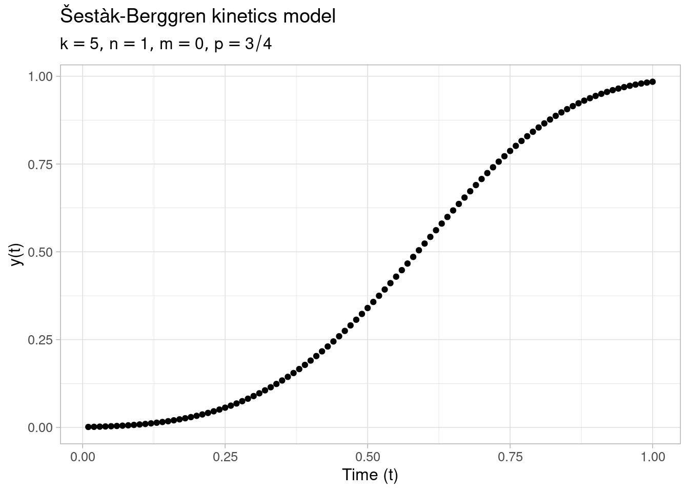
Analogous to the previous examples, using numerical differentiation of the gradients, we can fit the Šestàk-Berggren model to the generated data with the gsl_nls() function by:
## numeric differentiation
gsl_nls(
  fn = y ~ f(logk, n, m, p, times),               ## model formula
  data = data.frame(times = times, y = y),        ## model data
  start = list(logk = 0, n = 0, m = 0, p = 0),    ## starting values
  algorithm = "lm",                               ## levenberg-marquadt
  control = list(maxiter = 1e3)
)
#> Nonlinear regression model
#>   model: y ~ f(logk, n, m, p, times)
#>    data: data.frame(times = times, y = y)
#>    logk       n       m       p
#> 1.61360 0.97395 0.06779 0.68325
#>  residual sum-of-squares: 8.485e-07
#>
#> Algorithm: multifit/levenberg-marquardt, (scaling: more, solver: qr)
#>
#> Number of iterations to convergence: 44
#> Achieved convergence tolerance: 7.413e-14
We purposefully made a poor choice of parameter starting values and for this reason the optimized parameters do not correspond very well to the actual parameter values used to generate the data.
Proceeding with the Stan Math model implementation, the following C++ file encodes the Šestàk-Berggren model including evaluation of the Jacobian using reverse-mode AD and is compiled with Rcpp::sourceCpp():
// [[Rcpp::depends(BH)]]
// [[Rcpp::depends(RcppEigen)]]
// [[Rcpp::depends(RcppParallel)]]
// [[Rcpp::depends(StanHeaders)]]
#include <stan/math.hpp>
#include <Rcpp.h>
#include <RcppEigen.h>

// [[Rcpp::plugins(cpp14)]]

using namespace Rcpp;
using stan::math::exp;
using stan::math::fmax;
using stan::math::fmin;
using stan::math::log1m;
using stan::math::multiply_log;

struct kinetic_func {
    template <typename T_t, typename T_y, typename T_theta>
    Eigen::Matrix<stan::return_type_t<T_t, T_y, T_theta>, Eigen::Dynamic, 1>
    operator()(const T_t &t, const Eigen::Matrix<T_y, Eigen::Dynamic, 1> &y,
               std::ostream *msgs, const Eigen::Matrix<T_theta, Eigen::Dynamic, 1> &theta) const {

        Eigen::Matrix<T_y, Eigen::Dynamic, 1> dydt(1);

        T_y y1 = fmin(fmax(y(0), 1e-10), 1.0 - 1e-10); // constrain y to unit interval
        dydt << exp(theta(0) + theta(1) * log1m(y1) + multiply_log(theta(2), y1) + multiply_log(theta(3), -log1m(y1)));

        return dydt;
    }
};

// [[Rcpp::export]]
auto fjac_kinetic(double logk, double n, double m, double p, NumericVector ts)
{
    // initialization
    Eigen::Matrix<stan::math::var, Eigen::Dynamic, 1> theta(4);
    theta << logk, n, m, p;

    Eigen::VectorXd y0(1);
    y0 << 0.001;

    kinetic_func kf;

    // ode integration
    auto ys = stan::math::ode_rk45(kf, y0, 0, as<std::vector<double>>(ts), 0, theta);

    Eigen::VectorXd fx(ts.length());
    Eigen::MatrixXd jac_fx(4, ts.length());

    // response and jacobian
    for (int n = 0; n < ts.length(); ++n) {
        stan::math::set_zero_all_adjoints();
        ys[n](0).grad();
        fx(n) = ys[n](0).val();
        jac_fx.col(n) = theta.adj();
    }

    // reformat returned result
    NumericVector fx1 = wrap(fx);
    jac_fx.transposeInPlace();
    NumericMatrix jac_fx1 = wrap(jac_fx);
    colnames(jac_fx1) = CharacterVector({"logk", "n", "m", "p"});
    fx1.attr("gradient") = jac_fx1;

    return fx1;
}
Here, the ODE is integrated using the stan::math::ode_rk45() functional5. The derivative function of the ODE is passed to stan::math::ode_rk45() in the form of the functor kinetic_func. The functor only defines an operator() method, with a function signature as specified in the Stan Math function documentation6. The derivative function in the body of the operator() uses log1m and multiply_log for convenience, but other than that is equivalent to the expression used in deSolve::ode() above.
The vector of model parameters theta passed to stan::math::ode_rk45() is specified as an Eigen vector of type stan::math::var, which allows us to evaluate the time-specific gradients with respect to the parameters after solving the ODE. Instead of using the stan::math::jacobian() functional, the response vector and Jacobian matrix are populated by evaluating the reverse-mode gradient with .grad() applied to the ODE solution ys at each timepoint, and extracting the function values with .val() and the gradients with .adj() (applied to the parameter vector theta).
Remark: the functions fmax() and fmin() are not continuously differentiable with respect to their arguments. For automatic differentiation this is not necessarily an issue, but potential difficulties could arise in subsequent gradient-based optimization, as the gradient surface may not everywhere be a smooth function of the parameters. In this example, possible remedies could be replacing the hard cut-offs by smooth constraints or reparameterizing the model in such a way that the response is naturally constrained to the unit interval.
After compiling the C++ file, we refit the Šestàk-Berggren model to the generated data using the gsl_nls() function, but now with automatic differentiation to evaluate the Jacobian:
## automatic differentiation
gsl_nls(
  fn = y ~ fjac_kinetic(logk, n, m, p, times),
  data = data.frame(times = times, y = y),
  start = list(logk = 0, n = 0, m = 0, p = 0),
  algorithm = "lm",
)
#> Nonlinear regression model
#>   model: y ~ fjac_kinetic(logk, n, m, p, times)
#>    data: data.frame(times = times, y = y)
#>      logk         n         m         p
#> 1.6094332 0.9997281 0.0006153 0.7493653
#>  residual sum-of-squares: 3.675e-10
#>
#> Algorithm: multifit/levenberg-marquardt, (scaling: more, solver: qr)
#>
#> Number of iterations to convergence: 21
#> Achieved convergence tolerance: 4.897e-08
We observe that the estimated parameters have much better accuracy than in the previous model fit and also require less iterations to reach convergence. The number of iterations can further be reduced by switching to the Levenberg-Marquadt algorithm with geodesic acceleration (algorithm = "lmaccel"), which quickly converges to the correct solution:
## levenberg-marquardt w/ geodesic acceleration
gsl_nls(
  fn = y ~ fjac_kinetic(logk, n, m, p, times),
  data = data.frame(times = times, y = y),
  start = list(logk = 0, n = 0, m = 0, p = 0),
  algorithm = "lmaccel"
)
#> Nonlinear regression model
#>   model: y ~ fjac_kinetic(logk, n, m, p, times)
#>    data: data.frame(times = times, y = y)
#>       logk          n          m          p
#>  1.6093727  1.0001089 -0.0003747  0.7503401
#>  residual sum-of-squares: 9.04e-11
#>
#> Algorithm: multifit/levenberg-marquardt+accel, (scaling: more, solver: qr)
#>
#> Number of iterations to convergence: 12
#> Achieved convergence tolerance: 5.628e-09
Session Info
sessionInfo()
#> R version 4.1.1 (2021-08-10)
#> Platform: x86_64-pc-linux-gnu (64-bit)
#> Running under: Ubuntu 20.04.3 LTS
#>
#> Matrix products: default
#> BLAS:   /usr/lib/x86_64-linux-gnu/blas/libblas.so.3.9.0
#> LAPACK: /usr/lib/x86_64-linux-gnu/lapack/liblapack.so.3.9.0
#>
#> locale:
#>  [1] LC_CTYPE=en_US.UTF-8       LC_NUMERIC=C
#>  [3] LC_TIME=en_US.UTF-8        LC_COLLATE=en_US.UTF-8
#>  [5] LC_MONETARY=en_US.UTF-8    LC_MESSAGES=en_US.UTF-8
#>  [7] LC_PAPER=en_US.UTF-8       LC_NAME=C
#>  [9] LC_ADDRESS=C               LC_TELEPHONE=C
#> [11] LC_MEASUREMENT=en_US.UTF-8 LC_IDENTIFICATION=C
#>
#> attached base packages:
#> [1] stats     graphics  grDevices utils     datasets  methods   base
#>
#> other attached packages:
#> [1] deSolve_1.30  gslnls_1.1.1  Deriv_4.1.3   ggplot2_3.3.5 knitr_1.36
#>
#> loaded via a namespace (and not attached):
#>  [1] Rcpp_1.0.7          highr_0.9           bslib_0.3.1
#>  [4] compiler_4.1.1      pillar_1.6.3        jquerylib_0.1.4
#>  [7] tools_4.1.1         digest_0.6.29       lattice_0.20-45
#> [10] jsonlite_1.7.2      evaluate_0.14       lifecycle_1.0.1
#> [13] tibble_3.1.5        gtable_0.3.0        pkgconfig_2.0.3
#> [16] rlang_0.4.11        Matrix_1.4-0        yaml_2.2.1
#> [19] blogdown_1.5        xfun_0.26           fastmap_1.1.0
#> [22] withr_2.4.2         stringr_1.4.0       dplyr_1.0.7
#> [25] generics_0.1.0      sass_0.4.0          vctrs_0.3.8
#> [28] tidyselect_1.1.1    grid_4.1.1          glue_1.5.1
#> [31] R6_2.5.1            BH_1.75.0-0         fansi_0.5.0
#> [34] rmarkdown_2.11      bookdown_0.24       farver_2.1.0
#> [37] purrr_0.3.4         magrittr_2.0.1      StanHeaders_2.26.4
#> [40] scales_1.1.1        htmltools_0.5.2     ellipsis_0.3.2
#> [43] colorspace_2.0-2    labeling_0.4.2      utf8_1.2.2
#> [46] stringi_1.7.4       RcppParallel_5.1.4  munsell_0.5.0
#> [49] RcppEigen_0.3.3.9.1 crayon_1.4.1
References
see also the Using the Stan Math C++ Library vignette.↩︎
the evaluated gradient does not actually depend on the value of
theta, as the gradient does not contain any terms depending ontheta.↩︎the Watson function is still differentiable by hand, but manual derivation of complex nonlinear models in practice quickly becomes cumbersome (as well as error-prone).↩︎
the functor is defined in the form of a
struct, but could also be defined as aclass(with public methodoperator()).↩︎this functional requires
StanHeadersversion >= 2.24.↩︎the output stream pointer
std::ostream *msgscan be provided for messages printed by the integrator, but is not used here.↩︎